Section 9 Appendix 2: Data Pre-processing
Data preprocessing can be defined as the work required to turn raw data into the data used for modeling.
The raw data used in this analysis are remote sensing and other geographic information system data, hereafter “RS data,” such as digitized maps of elevation, population density, or public service locations. These data need to be aggregated and linked with the survey containing the data on the development indicators we plan to map.
Data preprocessing is arguably one of the most time-consuming tasks of any data science project. This section documents the path required to convert the raw data into data usable for high-resolution mapping. Here are the main steps:
- Load the RS layers.
- Create summaries for the RS layers that come with a time dimension (e.g., average precipitation over the last 30 years).
- Perform additional calculations as required (e.g., compute the soil degradation index based on soil degradation sub-indicator).
- Compute the distance metrics to public services, businesses, and some natural features.
- Align the coordinate reference systems (CRSs) across layers (geographic or projected).
- Aggregate the RS layers to the map of interest (e.g., the segmento map) with a chosen set of spatial statistics (e.g., average precipitation per segmento).
- Match the RS aggregates with the outcome data (poverty, income, literacy).
- Write the data frame to a
.csvfile for later use.
Readers interested in only the modeling instructions can skip this section entirely.
9.1 Data Sources
The 2017 EHPM household survey, collected by DIGESTYC, is used to compute the three main development indicators: median income, poverty, and literacy.
The EHPM survey data are stored in the file ehpm-2017.csv on the publicly available DIGESTYC website here. DIGESTYC provided the research team with the segmento identifiers, allowing the RS data to be linked with the EPHM data at the segmento level rather than the canton level, as would have been necessary if using only the publicly available data. The segmento identifier is stored in the file Identificador de segmento.xlsx.
A suite of RS data is used to determine potential predictors of the three main development indicators. The data sources are listed on the next table (see web-book version of this tutorial for the links).
| Names | Type | Source |
|---|---|---|
| Population count | raster | CIESIN |
| Precipitation | raster | Climate Hazards Center |
| Lights at night | raster | NOAA |
| Integrated Food Security Phase Classification | vector | FEWS NET |
| Livelihood zones | vector | FEWS NET |
| Altitude | raster | NASA Shuttle Radar Topography Mission (SRTMv003) |
| Soil degradation | raster | Trend.Earth |
| Buildings | vector | OpenStreetMap |
| Points of interest points | vector | OpenStreetMap |
| Roads network | vector | OpenStreetMap |
| Vegetation greenness (NDVI) | raster | U.S. Geological Survey (USGS) |
| Schools | vector | La Direccion General de Estadistica y Censos (DIGESTYC) |
| Health centers | csv | La Direccion General de Estadistica y Censos (DIGESTYC) |
| Hospitals | csv | La Direccion General de Estadistica y Censos (DIGESTYC) |
| Temperature | raster | WorldClim Version2 (Fick and Hijmans 2017) |
| Slope | raster | WorldPop Archive global gridded spatial datasets |
| Distance to OSM major roads | raster | WorldPop and CIESIN |
| Distance to OSM major roads intersections | raster | WorldPop and CIESIN |
| Distance to OSM major waterway | raster | WorldPop and CIESIN |
| Built settlement | raster | WorldPop and CIESIN |
| Land cover | raster | European Space Agency |
9.2 Loading the Survey
We start by loading the segmento shapefile and the EHPM survey data:
- ehpm: This is the EHPM survey data.
- segmento_hh_id: This is the segmento ID matched to the household ID, which allows us to map households at the segmento level.
- segmento shapefile: This is the map of all segmentos.
To create a more easily readable directory path, we create an object with the path to the folder where the data are stored:
9.3 Loading the Vectors
Vector data are polygons (e.g., administrative areas), lines (e.g., roads network), or points (e.g., coordinates of schools). They can be stored in various formats, with the most common being ESRI shapefiles and geojson files.
9.3.1 Loading the Administrative Boundaries
First, we load the administrative maps of the segmentos and departamentos with the command readOGR from the rgdal package. Shapefiles are loaded as a SpatialPolygonDataframe, which is a georeferenced set of polygons to which a data frame is attached.
dir_shape="spatial/shape/"
segmento_sh=readOGR(paste0(dir_data,
dir_shape,
"admin/STPLAN_Segmentos.shp"))## OGR data source with driver: ESRI Shapefile
## Source: "/home/rstudio/data/spatial/shape/admin/STPLAN_Segmentos.shp", layer: "STPLAN_Segmentos"
## with 12435 features
## It has 17 fields## OGR data source with driver: ESRI Shapefile
## Source: "/home/rstudio/data/spatial/shape/admin/STPLAN_Departamentos.shp", layer: "STPLAN_Departamentos"
## with 14 features
## It has 6 fieldsThesegmento_sh shape file loaded above, for example, consists of a data frame with 17 fields (variables).
The names of each field can be accessed by running this command:
## [1] "OBJECTID" "DEPTO" "COD_DEP" "MPIO" "COD_MUN"
## [6] "CANTON" "COD_CAN" "COD_ZON_CE" "COD_SEC_CE" "COD_SEG_CE"
## [11] "AREA_ID" "SEG_ID" "AREA_KM2" "SHAPE_Leng" "Shape_Le_1"
## [16] "Shape_Area" "demmean"The data frame attached to the polygon map can be inspected using the following functions:
## OBJECTID DEPTO COD_DEP MPIO COD_MUN CANTON COD_CAN COD_ZON_CE
## 0 1 AHUACHAPAN 01 ATIQUIZAYA 03 AREA URBANA 00 00
## 1 2 AHUACHAPAN 01 GUAYMANGO 06 EL ESCALON 04 00
## 2 3 AHUACHAPAN 01 AHUACHAPAN 01 AREA URBANA 00 01
## 3 4 AHUACHAPAN 01 AHUACHAPAN 01 AREA URBANA 00 01
## 4 5 AHUACHAPAN 01 AHUACHAPAN 01 AREA URBANA 00 02
## 5 6 AHUACHAPAN 01 AHUACHAPAN 01 AREA URBANA 00 02
## COD_SEC_CE COD_SEG_CE AREA_ID SEG_ID AREA_KM2 SHAPE_Leng Shape_Le_1
## 0 002 1015 U 01031015 0.04352 1261.0632 1261.0217
## 1 005 0016 R 01060016 1.65778 8536.1704 8535.8890
## 2 003 1015 U 01011015 0.07500 1165.9750 1165.9366
## 3 003 1014 U 01011014 0.05010 988.8543 988.8216
## 4 009 1019 U 01011019 0.06910 1135.7582 1135.7209
## 5 009 1042 U 01011042 0.04690 857.8403 857.8122
## Shape_Area demmean
## 0 43526.87 NA
## 1 1657675.21 NA
## 2 74995.98 NA
## 3 50104.03 NA
## 4 69104.02 NA
## 5 46899.53 NA## OBJECTID DEPTO COD_DEP MPIO
## Min. : 1 Length:12435 Length:12435 Length:12435
## 1st Qu.: 3110 Class :character Class :character Class :character
## Median : 6219 Mode :character Mode :character Mode :character
## Mean : 6219
## 3rd Qu.: 9328
## Max. :12437
##
## COD_MUN CANTON COD_CAN COD_ZON_CE
## Length:12435 Length:12435 Length:12435 Length:12435
## Class :character Class :character Class :character Class :character
## Mode :character Mode :character Mode :character Mode :character
##
##
##
##
## COD_SEC_CE COD_SEG_CE AREA_ID SEG_ID
## Length:12435 Length:12435 Length:12435 Length:12435
## Class :character Class :character Class :character Class :character
## Mode :character Mode :character Mode :character Mode :character
##
##
##
##
## AREA_KM2 SHAPE_Leng Shape_Le_1 Shape_Area
## Min. : 0.00000 Min. : 281.4 Min. : 281.4 Min. : 3903
## 1st Qu.: 0.06062 1st Qu.: 1256.3 1st Qu.: 1256.3 1st Qu.: 60567
## Median : 0.27345 Median : 2859.6 Median : 2859.5 Median : 273177
## Mean : 1.67100 Mean : 5494.0 Mean : 5493.8 Mean : 1672961
## 3rd Qu.: 2.08214 3rd Qu.: 8492.5 3rd Qu.: 8492.3 3rd Qu.: 2082009
## Max. :48.36518 Max. :54684.4 Max. :54682.6 Max. :48194678
##
## demmean
## Min. : NA
## 1st Qu.: NA
## Median : NA
## Mean :NaN
## 3rd Qu.: NA
## Max. : NA
## NA's :12435We see that Shape_Le_1 and SHAPE_Leng are duplicates, while demmean comprises only null values. These fields are removed using the dplyr function select.
To get a country mask, which is the boundary of the country, we dissolve the multiple polygons of the departamentos shapefile into one overall map of the country with the function maptools::unionSpatialPolygons.
The country mask is shown in Figure 9.1.
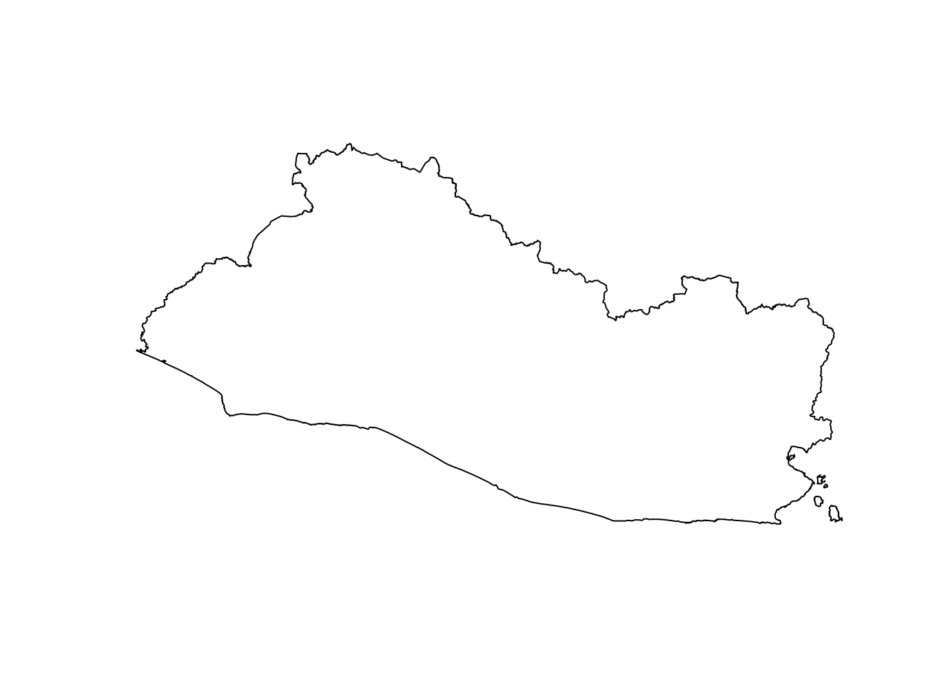
Figure 9.1: El Salvador country mask
9.3.1.1 Adjusting the Coordinates System
There are two families of coordinates systems:
- Geographic coordinate systems (GCS): “A system that uses a three-dimensional spherical surface to define locations on the earth.”5.
- Projected coordinate systems (PCS): “A system defined on a flat, two-dimensional surface. Unlike a geographic coordinate system, a projected coordinate system has constant lengths, angles, and areas across the two dimensions.”6
The shapefiles for the segmentos, departmentos, and the country mask have a projected coordinate system.
## CRS arguments:
## +proj=lcc +lat_0=13.783333 +lon_0=-89 +lat_1=13.316666 +lat_2=14.25
## +x_0=500000 +y_0=295809.184 +k_0=0.99996704 +datum=NAD27 +units=m
## +no_defsThe coordinates are expressed in meters:
## min max
## x 377579.6 642687.1
## y 226506.1 369595.5Since most spatial RS data are based on a GCS, we create a second version of the country mask with one. This is done with the function spTransform from the sp library. The use of :: allows us to call the function without loading the sp library in the environment.
proj_WGS_84="+proj=longlat +datum=WGS84 +no_defs +ellps=WGS84 +towgs84=0,0,0"
segmento_sh_wgs=sp::spTransform(segmento_sh,
proj_WGS_84)## Warning in showSRID(uprojargs, format = "PROJ", multiline = "NO"): Discarded datum WGS_1984 in CRS definition,
## but +towgs84= values preserved## Warning in showSRID(uprojargs, format = "PROJ", multiline = "NO"): Discarded datum WGS_1984 in CRS definition,
## but +towgs84= values preserved## min max
## x -90.13200 -87.68380
## y 13.15541 14.45093The coordinates are now expressed in decimal degrees.
9.3.2 Loading the Shapefiles Containing the Fields Used as Covariates
We now load the shapefiles containing the fields used as covariates, which are the containing variables that will be used as predictors in the model we will fit in the next sections.
We start with the Livelihood zone maps accessed from the Famine Early Warning Systems Network (FEWS NET).
The livelihood zone map is mapped on 9.2 for inspection.
leaflet(LZ_sh)%>%
addTiles()%>%
addPolygons(weight=1,
color = "#444444",
smoothFactor = 1,
fillOpacity = 1,
fillColor = ~colorFactor("Accent", LZNAMEEN)(LZNAMEEN),
popup = ~LZNAMEEN)%>%
addLegend("bottomright",
colors = ~colorFactor("Accent", LZNAMEEN)(LZNAMEEN),
labels = ~LZNAMEEN,
opacity = 1)Figure 9.2: Livelihood zones
Next, we load all the other Vectors data.
school_sh=readOGR(paste0(dir_data,
dir_shape,
"schools/MINED.shp"),use_iconv=TRUE, encoding = "UTF-8")
buildings_poly_sh=readOGR(paste0(dir_data,
dir_shape,
"hotosm/hotosm_slv_buildings_polygons.shp"), use_iconv=TRUE)
poi_points_sh=readOGR(paste0(dir_data,
dir_shape,
"hotosm/hotosm_slv_points_of_interest_points.shp"))
poi_poly_sh=readOGR(paste0(dir_data,
dir_shape,
"hotosm/hotosm_slv_points_of_interest_polygons.shp"))
roads_lines_sh=readOGR(paste0(dir_data,
dir_shape,
"hotosm/hotosm_slv_roads_lines.shp"))
roads_poly_sh=readOGR(paste0(dir_data,
dir_shape,
"hotosm/hotosm_slv_roads_polygons.shp"))
coastline=readOGR(paste0(dir_data,
dir_shape,
"coastline/coastline.shp"))
waterbodies=readOGR(paste0(dir_data,
dir_shape,
"hotosm/hotosm_slv_waterways_polygons.shp"))
proj_lcc=" +proj=lcc +lat_1=13.316666 +lat_2=14.25 +lat_0=13.783333 +lon_0=-89 +x_0=500000 +y_0=295809.184 +datum=NAD27 +units=m +no_defs +ellps=clrk66 +nadgrids=@conus,@alaska,@ntv2_0.gsb,@ntv1_can.dat"
# waterbodies_proj=sp::spTransform(waterbodies,
# proj_lcc)
waterbodies_proj= waterbodies
rivers=readOGR(paste0(dir_data,
dir_shape,
"hotosm/hotosm_slv_waterways_lines.shp"))
# rivers_proj=sp::spTransform(rivers,
# proj_lcc)
rivers_proj=rivers9.3.3 Loading Point-Referenced Data from Tables
Two datasets are provided as R data frames in a .Rda file. They are loaded with the function load:
load(paste0(dir_data,
dir_shape,
"hospitales/hospitales.Rda"))
load(paste0(dir_data,
dir_shape,
"UCSF/UCSF.Rda"))The package sp is then used to turn the data frames into SpatialPointsDataframe objects.
# In the .Rda, there is an error in the naming of the coordinates: latitudes are actually longitudes and vice versa
hospitales=hospitales%>%
rename(lon=latitude,
lat=longitude)
hospitals_sp=as.data.frame(hospitales)
# Features "lon" and "lat" are declared the the spatial coordinates of the data frame "hospitals_sp"
# The data frame "hospitals_sp" becomes an object of the type SpatialPointsDataframe
sp::coordinates(hospitals_sp)=~lon+lat
# A spatial coordinate system is assigned to the SpatialPointsDataframe "hospitals_sp"
sp::proj4string(hospitals_sp)=sp::CRS(proj_WGS_84)## Warning in showSRID(uprojargs, format = "PROJ", multiline = "NO"): Discarded datum WGS_1984 in CRS definition,
## but +towgs84= values preservedThe same is done with the health center (not shown).
The resulting map is plotted on 9.3 for reference.7
leaflet(SLV_adm0)%>%
addPolygons()%>%
addTiles()%>%
addMarkers(lng=coordinates(hospitals_sp)[,1],
lat=coordinates(hospitals_sp)[,2],
popup=hospitals_sp$name)%>%
addCircleMarkers(lng=coordinates(health_centres_sp)[,1],
lat=coordinates(health_centres_sp)[,2],
radius = 4,
popup=paste0(health_centres_sp$name,"\n(",health_centres_sp$tipo,")"),
stroke = F,
fillOpacity = 1,
fillColor = colorFactor("Accent", health_centres_sp$tipo)(health_centres_sp$tipo))Figure 9.3: Health Centers
9.4 Loading the Rasters
We now turn to the raster files. Raster files can be described as georeferenced pixel data. For instance, a raster of population density consists of a map of pixels. The value of each pixel is the density of people in this pixel. The two main formats for raster data are zipped .tif and .ncdf files.
9.4.1 Lights at Night
Lights at night data products are available by calendar month and year. In this tutorial, annual data are used for 1983 to 2016. The yearly aggregate data for 2017 had not yet been released when we began data preprocessing, so monthly aggregated data were used.
The first step is to unzip the files with the untar command. For the sake of convenience, the data are already provided as extracted .tif in the data folder data/spatial/raster/l@n/, so the code snippet below is just shown for illustrative purposes and does not need to be run.
# Get the list of all files in the l@n directory with the command -dir-, which takes as argument
# The path to the directory
list_of_files=dir(paste0(dir_data,
"spatial/raster/l@n/"))
# Identify the index of the 2017 monthly files
index_of_2017_files=grep("npp_2017",
dir(paste0(dir_data,
"spatial/raster/l@n/")))
# Selecting in the list of all files the 2017 monthly files thanks to the index
files_2017=list_of_files[index_of_2017_files]
# for(monthly_file in files_2017){
# untar(paste0(dir_data,
# "spatial/raster/l@n/",
# monthly_file), # The path to the file of interest
# compressed="gzip", # Specify it was zipped with gzip
# exdir=paste0(dir_data,
# "spatial/raster/l@n/")) # Specify the directory where the files need to be unzipped exdir
# }The 12 monthly lights at night .tif files are loaded with the raster::raster function, cropped to El Salvador’s boundaries with raster::crop, and stacked in one object with raster::stack. Note the use of the for loop function to loop the 12 monthly files.
# Get the list of the files in the directory
list_of_files=dir(paste0(dir_data,
"spatial/raster/l@n/"))
# Get the list of lights at night files labelled "avg_rade9h"
monthly_file_light=list_of_files[grepl("avg_rade9h",
list_of_files,
fixed=T)]
# Create a vector of character to name the raster as file_1, file_2, etc.
names_file=paste0("file_",1:12)
# Loop over the 12 monthly files in order to:
for(i in 1:length(monthly_file_light)){
# Load each i monthly layer
r=raster::raster(paste0(dir_data,
"spatial/raster/l@n/",
monthly_file_light[i]))
# Crop each i monthly layer
r=raster::crop(r,
SLV_adm0)
# Assign each i cropped monthly layer to a name
assign(names_file[i], # assign it to an object name
r)
}
# Stack all the layers
lights_all=raster::stack(lapply(names_file,FUN=get)) Let us have a look at the object lights_all:
## [1] "RasterStack"## [1] 311 587 12## [1] 0.004166667 0.004166667## class : Extent
## xmin : -90.13125
## xmax : -87.68542
## ymin : 13.15625
## ymax : 14.45208## CRS arguments: +proj=longlat +datum=WGS84 +no_defsThis a RasterStack object, which is a stack of rasters where each layer is aligned above another, with 310 rows, 587 columns, and 12 layers (1 per month) for a total of 181,970 cells. The resolution is provided in decimal degrees: 0.004166667 degrees by 0.004166667 degrees pixels.
Next, we plot the 12 monthly layers for inspection.
raster::plot(lights_all,
main=c("jan","feb","mar","apr","may","jun","jul","aug","sep","oct","nov","dec"))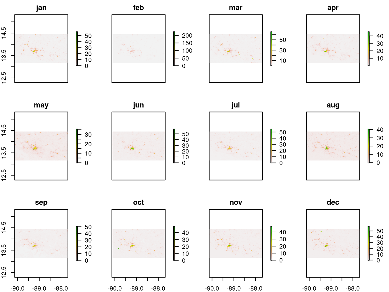
Figure 9.4: 2017 monthly average lights at night (average DNB radiance)
The maps in 9.4 show there are variations over the year.
9.4.2 Precipitation
The CHIRPS precipitation data are provided as an .nc file, which is a collection of raster files similar to a raster stack. Data are loaded as a brick using the raster::brick function, similar to the raster stack function.8
chirps=raster::brick(paste0(dir_data,
"spatial/raster/chirps/chirps-v2.0.annual.nc"),
band=1:38)
print(chirps)## File /home/rstudio/data/spatial/raster/chirps/chirps-v2.0.annual.nc (NC_FORMAT_NETCDF4):
##
## 1 variables (excluding dimension variables):
## float precip[longitude,latitude,time] (Chunking: [800,223,4]) (Compression: level 5)
## units: mm/year
## standard_name: convective precipitation rate
## long_name: Climate Hazards group InfraRed Precipitation with Stations
## time_step: year
## missing_value: -9999
## _FillValue: -9999
## geostatial_lat_min: -50
## geostatial_lat_max: 50
## geostatial_lon_min: -180
## geostatial_lon_max: 180
##
## 3 dimensions:
## longitude Size:7200
## units: degrees_east
## standard_name: longitude
## long_name: longitude
## axis: X
## latitude Size:2000
## units: degrees_north
## standard_name: latitude
## long_name: latitude
## axis: Y
## time Size:38
## units: days since 1980-1-1 0:0:0
## standard_name: time
## calendar: gregorian
## axis: T
##
## 15 global attributes:
## Conventions: CF-1.6
## title: CHIRPS Version 2.0
## history: created by Climate Hazards Group
## version: Version 2.0
## date_created: 2019-01-30
## creator_name: Pete Peterson
## creator_email: pete@geog.ucsb.edu
## institution: Climate Hazards Group. University of California at Santa Barbara
## documentation: http://pubs.usgs.gov/ds/832/
## reference: Funk, C.C., Peterson, P.J., Landsfeld, M.F., Pedreros, D.H., Verdin, J.P., Rowland, J.D., Romero, B.E., Husak, G.J., Michaelsen, J.C., and Verdin, A.P., 2014, A quasi-global precipitation time series for drought monitoring: U.S. Geological Survey Data Series 832, 4 p., http://dx.doi.org/110.3133/ds832.
## comments: time variable denotes the first day of the given year.
## acknowledgements: The Climate Hazards Group InfraRed Precipitation with Stations development process was carried out through U.S. Geological Survey (USGS) cooperative agreement #G09AC000001 "Monitoring and Forecasting Climate, Water and Land Use for Food Production in the Developing World" with funding from: U.S. Agency for International Development Office of Food for Peace, award #AID-FFP-P-10-00002 for "Famine Early Warning Systems Network Support," the National Aeronautics and Space Administration Applied Sciences Program, Decisions award #NN10AN26I for "A Land Data Assimilation System for Famine Early Warning," SERVIR award #NNH12AU22I for "A Long Time-Series Indicator of Agricultural Drought for the Greater Horn of Africa," The National Oceanic and Atmospheric Administration award NA11OAR4310151 for "A Global Standardized Precipitation Index supporting the US Drought Portal and the Famine Early Warning System Network," and the USGS Land Change Science Program.
## ftp_url: ftp://chg-ftpout.geog.ucsb.edu/pub/org/chg/products/CHIRPS-latest/
## website: http://chg.geog.ucsb.edu/data/chirps/index.html
## faq: http://chg-wiki.geog.ucsb.edu/wiki/CHIRPS_FAQThe raster chirps provides global annual cumulative precipitation over 38 years (38 bands), from 1981 to 2018, at a resolution of 0.05 longitude/latitude decimal degrees.
Next, the data are cropped to El Salvador’s borders, and all years until 2017 are selected (data are provided up to January 2018 in the file).
# Crop the data
chirps_ev=raster::crop(chirps,
SLV_adm0)
time = raster::getZ(chirps_ev) # get the time index
index_of_1981_2017 = which(dplyr::between(time,
as.Date("1981-01-01"),
as.Date("2017-01-01")))
index_of_2017 = which(time==as.Date("2017-01-01"))
# Subset the CHIRPS to 1981–2017 (take out 2018)
chirps_ev_1981_2017=raster::subset(chirps_ev,
index_of_1981_2017)9.4.3 Soil Degradation
The soil degradation data were obtained via the QGIS plugin tool TRENDS.EARTH.9 The three main soil-degradation indexes provided in the TRENDS.EARTH are soil carbon stock degradation, the soil land-use change degradation, and soil productivity degradation, which has subindexes called trajectory, performance, and state.
Data for each of the above are provided in a series of multilayer .tif files. The .json file provides information about each layer.
soil_deg_carb_path="spatial/raster/soil_deg_carb/soil_deg_carb.json"
soil_deg_carb_json=RJSONIO::fromJSON(paste0(dir_data,
soil_deg_carb_path))
grep("degradation",
lapply(lapply(soil_deg_carb_json$bands,
unlist),
cbind))
soil_deg_luc_json_path="spatial/raster/soil_deg_luc/soil_deg_luc.json"
soil_deg_luc_json=RJSONIO::fromJSON(paste0(dir_data,
soil_deg_luc_json_path))
lapply(lapply(soil_deg_luc_json$bands,
unlist),
cbind)
grep("degradation",
lapply(lapply(soil_deg_luc_json$bands,
unlist),
cbind))
soil_deg_prod_json_path="spatial/raster/soil_deg_prod/soil_deg_prod.json"
soil_deg_prod_json=RJSONIO::fromJSON(paste0(dir_data,
soil_deg_prod_json_path))
grep("degradation",
lapply(lapply(soil_deg_prod_json$bands,
unlist),
cbind))For the carbon and land-use change files, band 1 provides the soil degradation index. For the productivity file, the index values on the trajectory, performance, and state are stored in bands 2, 4, and 7.
soil_deg_carb_path="spatial/raster/soil_deg_carb/soil_deg_carb.tif"
soil_deg_carb=raster::raster(paste0(dir_data,
soil_deg_carb_path),
band=1) # Soil degradation, change in the carbon method
soil_deg_luc_path="spatial/raster/soil_deg_luc/soil_deg_luc.tif"
soil_deg_luc=raster::raster(paste0(dir_data,
soil_deg_luc_path),
band=1) # Soil degradation, land use change
soil_deg_prod_trj_path="spatial/raster/soil_deg_prod/soil_deg_prod.tif"
soil_deg_prod_trj=raster::raster(paste0(dir_data,
soil_deg_prod_trj_path),
band=2) # Soil degradation, productivity trajectory deg
soil_deg_prod_prf_path="spatial/raster/soil_deg_prod/soil_deg_prod.tif"
soil_deg_prod_prf=raster::raster(paste0(dir_data,
soil_deg_prod_prf_path),
band=4) # Soil degradation, productivity performance deg
soil_deg_prod_stt_path="spatial/raster/soil_deg_prod/soil_deg_prod.tif"
soil_deg_prod_stt=raster::raster(paste0(dir_data,
soil_deg_prod_stt_path),
band=7) # Soil degradation, productivity state deg9.4.4 Vegetation Greenness
Vegetation greenness data, as measured by normalized difference vegetation index, are provided on a dekadal (every 10 days) basis. Two data products are available: the smoothed dekadal NDVI value for 2017, and the median dekadal NDVI value over the period 2003–2017.
The first step is to unzip the data with the following code snippet. For the sake of convenience, the data are provided as unzipped .tif in the data pack, but the code to unzip the files is also provided below.
# Get the list of all files in the ndvi directory with the command -dir-
list_of_files=dir(paste0(dir_data,
"spatial/raster/ndvi/"))
# Identify the index of the 2017 monthly files and norma
index_of_2017_std_files=grep("17|stm",
dir(paste0(dir_data,
"spatial/raster/ndvi/")))
# Select in the list of all file the 2017 monthly files thanks to the index
files_of_interest=list_of_files[index_of_2017_std_files]
# for(file in files_of_interest){
# untar(paste0(dir_data,
# "spatial/raster/ndvi/",
# file), # The path to the file of interest
# compressed="gzip",
# exdir=paste0(dir_data,
# "spatial/raster/ndvi/"))
# }The data are then loaded. Note the use of the function grep and the regular expressions to flexibly select the appropriate set of files:
"ca17[[:digit:]]{2}.tif"means: “ca17”, followed by a suite of 2 digits, followed by “.tif” -> these are the 2017 files"ca[[:digit:]]{2}stm.tif"means: “ca”, followed by a suite of 2 digits, followed by “stm.tif” -> these are the median files
# Create a vector of character to name the raster as ndvi_1, ndvi_2, etc.
names_ndvi_17=paste0("ndvi_",1:36)
names_ndvi_norm=paste0("ndvi_norm_",1:36)
# List of the 36 dekadal file for 2017 thanks to the command -grep- and the regular expression
list_of_files=dir(paste0(dir_data,
"spatial/raster/ndvi/"))
files_17=list_of_files[grep("ca17[[:digit:]]{2}.tif",
list_of_files)]
# The list of 36 ones for the 2003–2017 median
files_norm=list_of_files[grep("ca[[:digit:]]{2}stm.tif",
list_of_files)]
# Loop the 36 dekadal 2017 and normal files to load and crop them
for(i in 1:length(files_17)){
# 1) The 2017 data:
# Load each i dekadal layer
r=raster::raster(paste0(dir_data,
"spatial/raster/ndvi/",
files_17[i]))
# Crop each i monthly layer
r=raster::crop(r,
SLV_adm0)
# Assign each i cropped monthly layer to a name
assign(names_ndvi_17[i], # assign it to an object name
r)
# 2) The median data
# Load each i dekadal layer
r=raster::raster(paste0(dir_data,
"spatial/raster/ndvi/",
files_norm[i]))
# Crop each i monthly layer
r=raster::crop(r,
SLV_adm0)
# Assign each i cropped monthly layer to a name
assign(names_ndvi_norm[i], # Assign it to an object name
r)
}
# Stack all the layers
ndvi_17=raster::stack(lapply(names_ndvi_17,
FUN=get))
ndvi_norm=raster::stack(lapply(names_ndvi_norm,
FUN=get)) The rasters are then resampled to perfectly align both sets:
9.4.5 Temperature
The 12 monthly average temperature data rasters are cropped and stacked.
files_temp=dir(paste0(dir_data,
"spatial/raster/temperature/"))[grep("wc2.0_30s_tavg_",
dir(paste0(dir_data,
"spatial/raster/temperature/")))]
month=1
for(temp_m in files_temp){
temp=raster::raster(paste0(dir_data,
"spatial/raster/temperature/",temp_m))
temp=raster::crop(temp,
SLV_adm0)
assign(paste0("temp_",month),
temp)
month=month+1
}
temp_months=raster::stack(lapply(paste0("temp_",
1:12),
FUN=get))9.4.6 Slope
The slope data are obtained from the WorldPop Dataverse Repository as a suite of raster files, each of which covers a portion of El Salvador’s territory. The rasters are combined into a single raster to ease preprocessing work.
slope_files=paste0(dir_data,
"spatial/raster/slope/",
dir(paste0(dir_data,
"spatial/raster/slope/")))
i=1
raster_list=list()
for(file in slope_files){
raster_f=raster::raster(file)
raster_list[[i]]=raster_f
i=i+1
}
slope <- do.call(raster::merge, raster_list)
slope=raster::crop(slope,
SLV_adm0)
raster::plot(slope,
main="Slope (degrees)")
sp::plot(SLV_adm0,
add=T)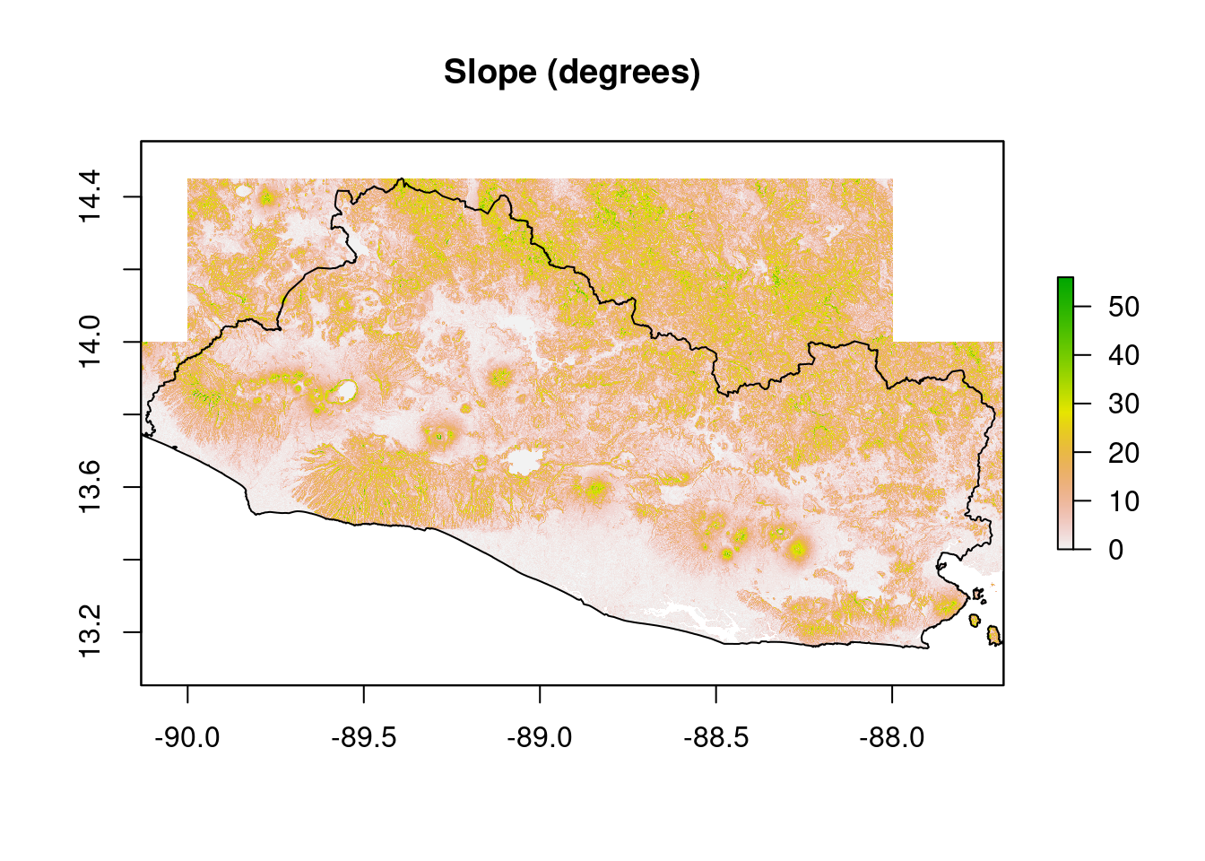
9.4.7 Other Rasters
The other rasters are loaded with the function raster:
dem=raster::raster(paste0(dir_data,
"spatial/raster/dem/srtm_dem.tif"))
dist2road_path="spatial/raster/distance2roads/slv_osm_dst_road_100m_2016.tif"
dist2road=raster::raster(paste0(dir_data,
dist2road_path))
dist2roadInter_path="spatial/raster/distance2intersections/slv_osm_dst_roadintersec_100m_2016.tif"
dist2roadInter=raster::raster(paste0(dir_data,
dist2roadInter_path))
settlements_path="spatial/raster/settlements/slv_bsgme_v0a_100m_2017.tif"
settlements=raster::raster(paste0(dir_data,
settlements_path))
dist2water_path="spatial/raster/distance2waterway/slv_osm_dst_waterway_100m_2016.tif"
dist2water=raster::raster(paste0(dir_data,
dist2water_path))
gpw_path="spatial/raster/GPW/gpw_v4_population_count_adjusted_to_2015_unwpp_country_totals_rev11_2015_30_sec.tif"
gpw=raster::raster(paste0(dir_data,gpw_path)) # Population count for 2015
gpw_es=raster::crop(gpw,
SLV_adm0)
lc_path="spatial/raster/CCILC/ESACCI-LC-L4-LCCS-Map-300m-P1Y-2015-v2.0.7_sv.tif"
lc=raster::raster(paste0(dir_data,lc_path)) # Land classWe can plot these rasters for quality controls. Figure 9.5 shows the digital elevation model, that is, altitudes across the country.
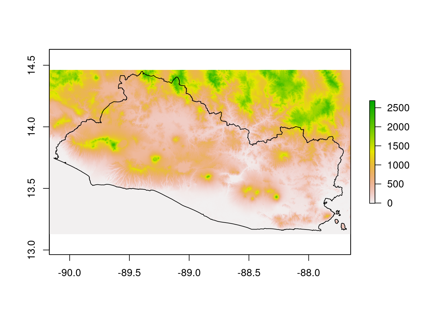
Figure 9.5: Digital Elevation Model
Figure 9.6 shows the population density data. By examining the GPW data, it is possible to identify some geometric forms corresponding to the enumeration areas of the census.
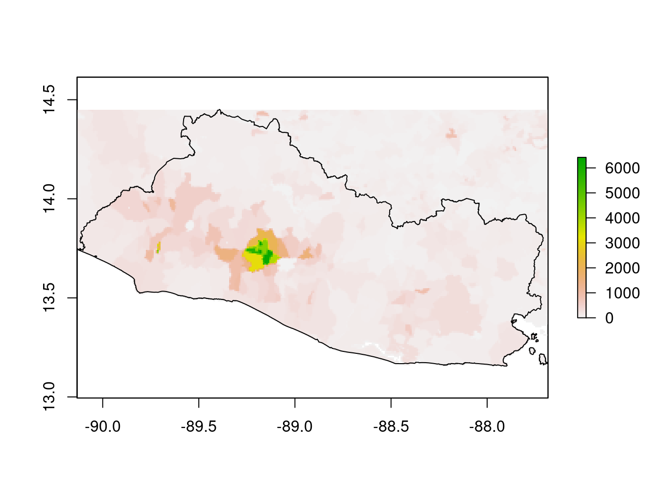
Figure 9.6: Population density data (GPW)
9.5 Rasters Calculation
The lights at night raster is expected to be a good predictor of economic activity (Henderson and Weil 2012). However, it is not clear which summary statistics will best predict the three development indicators. For example, we cannot establish with certainty whether annual average lights at night or annual minimum average monthly lights at night is a better predictor of poverty. This holds for the other raster data as well.
9.5.1 Lights at Night
The median and standard deviation of the lights at night data are computed for each map pixel:
lights_med=raster::calc(lights_all,
fun = median,
na.rm = T)
lights_sd=raster::calc(lights_all,
fun = sd,
na.rm = T)
lights_summaries=raster::stack(lights_med,
lights_sd)
names(lights_summaries)=c("lights_med",
"lights_sd")The results are plotted in Figure 9.7.
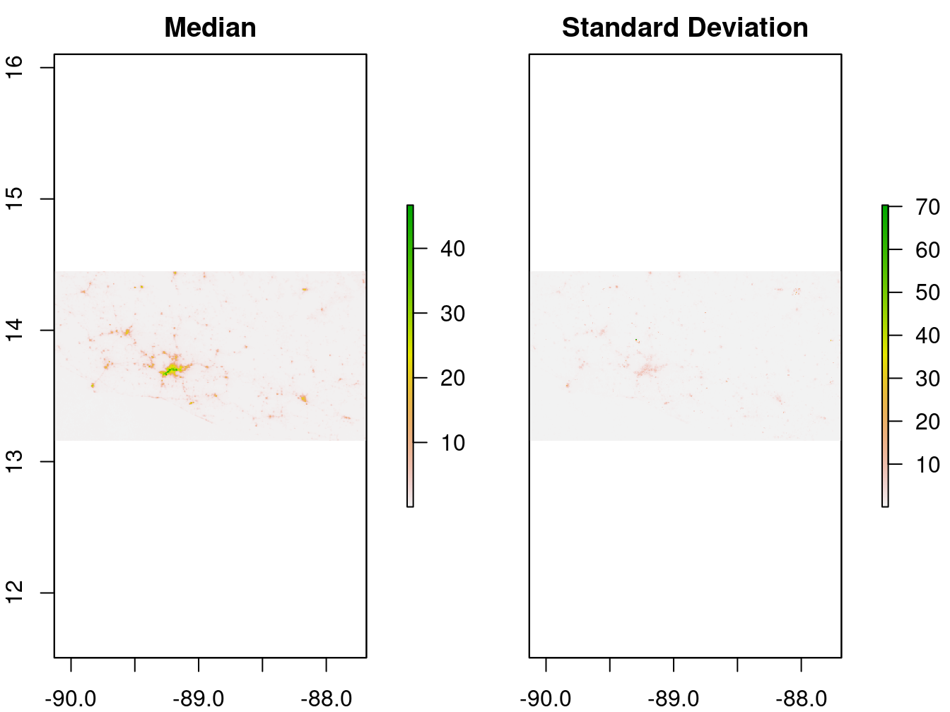
Figure 9.7: 2017 monthly average lights at night (average DNB radiance)
9.5.2 Precipitation
Again, as it is not clear a priori which summary statistics of precipitation are best at predicting the development indicators, a series of summary statistics is computed for each pixel of the map:
- Two precipitation summaries related to short-term weather:
- Annual cumulative precipitation for 2017
- Annual cumulative precipitation for 2017 as a percentage of normal
- Two precipitation summaries related to climate:
- Median annual cumulative precipitation over the 38-year period
- Standard deviation in precipitation between years
# Compute summaries
chirps_ev_2017=raster::subset(chirps_ev,
index_of_2017) # 2017
chirps_ev_med=raster::calc(chirps_ev_1981_2017,
fun = median,
na.rm = T) #medi
chirps_summaries=raster::stack(chirps_ev_2017,
chirps_ev_med)
names(chirps_summaries)=c("chirps_ev_2017",
"chirps_ev_med")For quality control, we plot the respective summaries.
raster::plot(chirps_summaries,
main=c("2017 precipitation",
"2017 precipitation as percentage of normal",
"1981-2017 median",
"1981-2017 standard deviation"))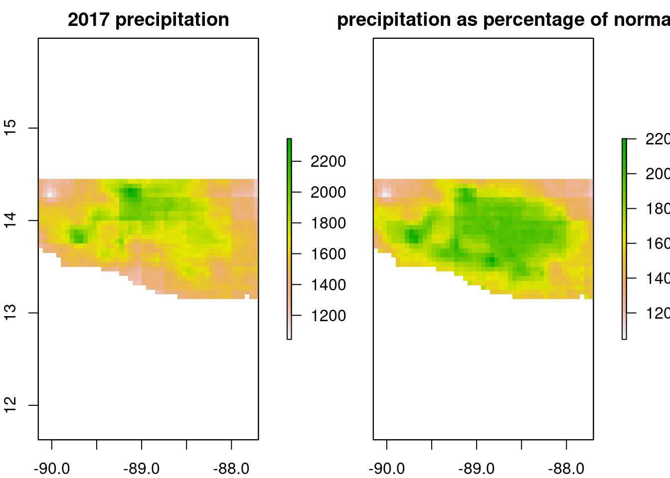
9.5.3 Vegetation Greenness
Various statistics are computed on the dekadal NDVI and its deviation from the 2003–2017 normal (median pixel value over the period).
ndvi_17_perc=(ndvi_17_re/ndvi_norm)*100
# annual NDVI values
ndvi_17_sum=raster::calc(ndvi_17_re,
fun = sum,
na.rm = T)
ndvi_17_summaries=raster::stack(ndvi_17_sum)
names(ndvi_17_summaries)=c("ndvi_17_sum")
# NDVI as a percentage of the 2003–2017 norm
ndvi_17_perc_sum=raster::calc(ndvi_17_perc,
fun = sum,
na.rm = T)
ndvi_17_perc_summaries=raster::stack(ndvi_17_perc_sum)
names(ndvi_17_perc_summaries)=c("ndvi_17_perc_sum")9.5.4 Soil Degradation
The missing data are stored in the raw rasters as -32768 and turned into NA. Next, the soil degradation data are simplified by creating one binary raster for the three soil degradation proxies: the soil is degraded or not.
# Soil carbon stock degradation
# Replace the NA
soil_deg_carb_val=raster::getValues(soil_deg_carb)
index_na=which(soil_deg_carb_val==-32768)
soil_deg_carb_val[index_na]=NA #set to NA the cell identified with original value of -32768
# Binarize for degradation
index_deg=which(soil_deg_carb_val<0)
soil_deg_carb_deg=soil_deg_carb_val
soil_deg_carb_deg[index_deg]=1
soil_deg_carb_deg[-index_deg]=0
soil_deg_carb_deg[index_na]=NA
soil_deg_carb_deg=raster::setValues(soil_deg_carb,
soil_deg_carb_deg) As the code is quite lengthy, it is shown only for the carbon stock soil degradation process.
# Soil Land use change degradation
soil_deg_luc_val=raster::getValues(soil_deg_luc)
index_deg=which(soil_deg_luc_val<0)
soil_deg_luc_deg=soil_deg_luc_val
soil_deg_luc_deg[index_deg]=1
soil_deg_luc_deg[-index_deg]=0
soil_deg_luc_deg=raster::setValues(soil_deg_luc,
soil_deg_luc_deg)
# Soil Productivity degradation
# Trajectory
soil_deg_prod_trj_val=raster::getValues(soil_deg_prod_trj)
index_na=which(soil_deg_prod_trj_val==-32768)
index_deg=which(soil_deg_prod_trj_val<0)
soil_deg_prod_trj_val[index_na]=NA
soil_deg_prod_trj_deg=soil_deg_prod_trj_val
soil_deg_prod_trj_deg[index_deg]=1
soil_deg_prod_trj_deg[-index_deg]=0
soil_deg_prod_trj_deg[index_na]=NA
soil_deg_prod_trj_deg=raster::setValues(soil_deg_prod_trj,
soil_deg_prod_trj_deg)
# Performance
soil_deg_prod_prf_val=raster::getValues(soil_deg_prod_prf)
index_na=which(soil_deg_prod_prf_val==-32768)
index_deg=which(soil_deg_prod_prf_val<0)
soil_deg_prod_prf_val[index_na]=NA
soil_deg_prod_prf_deg=soil_deg_prod_prf_val
soil_deg_prod_prf_deg[index_deg]=1
soil_deg_prod_prf_deg[-index_deg]=0
soil_deg_prod_prf_deg[index_na]=NA
soil_deg_prod_prf_deg=raster::setValues(soil_deg_prod_prf,
soil_deg_prod_prf_deg)
# State
soil_deg_prod_stt_val=raster::getValues(soil_deg_prod_stt)
index_na=which(soil_deg_prod_stt_val==-32768)
index_deg=which(soil_deg_prod_stt_val<0)
soil_deg_prod_stt_val[index_na]=NA
soil_deg_prod_stt_deg=soil_deg_prod_stt_val
soil_deg_prod_stt_deg[index_deg]=1
soil_deg_prod_stt_deg[-index_deg]=0
soil_deg_prod_stt_deg[index_na]=NA
soil_deg_prod_stt_deg=raster::setValues(soil_deg_prod_stt,
soil_deg_prod_stt_deg) Finally, the SDG Indicator (15.3) for soil degradation indicator is computed. It is based on the one-out-all-out principle that is, if a pixel is considered as soil degraded in any of the three soil degradation layers, then it is considered degraded in the SDG indicator.
The first step consists of aligning the raster to make sure the pixels of each layer are perfectly overlaid.
# Check that the rasters' extents are the same
all(raster::extent(soil_deg_luc_deg)==raster::extent(soil_deg_prod_stt_deg),
raster::extent(soil_deg_carb_deg)==raster::extent(soil_deg_prod_stt_deg))## [1] FALSEAs some of the layers have a slightly different extent, the values of each layer are resampled in the same raster grid.
# Resample the raster "soil_deg_luc_deg" to the same resolution and extent than the raster "soil_deg_prod_stt_deg"
soil_deg_luc_deg_re=raster::resample(soil_deg_luc_deg,
soil_deg_prod_stt_deg)
# Round the value, as the resampling takes averages while we want 0/1
soil_deg_luc_deg_re_val=raster::getValues(soil_deg_luc_deg_re)
soil_deg_luc_deg_re_val_r=round(soil_deg_luc_deg_re_val)
soil_deg_luc_deg_re_r=raster::setValues(soil_deg_luc_deg_re,
soil_deg_luc_deg_re_val_r)
raster::plot(soil_deg_luc_deg_re_r)
sp::plot(SLV_adm0,
add=T)
The same is done with the raster soil_deg_carb_deg (not shown).
The resulting rasters are stacked, and the SDG index is computed.
# Stack the rasters ####
soil_deg=raster::stack(soil_deg_carb_deg_re_r,
soil_deg_luc_deg_re_r,
soil_deg_prod_stt_deg,
soil_deg_prod_prf_deg,
soil_deg_prod_trj_deg)
names(soil_deg)=c("soil_carb",
"soil_luc",
"soil_prod_state",
"soil_prod_prf",
"soil_prod_trj")
# SDG 15.3.1 soil degradation index (one out all out principle) ####
soil_deg_SDG_index=raster::calc(soil_deg,
sum,
na.rm=T)
soil_deg_SDG_index=raster::calc(soil_deg_SDG_index,
fun=function(x) {x[x>0] = 1; return(x)}
)And here is the map of soil degradation according to SDG Indicator 15.3:
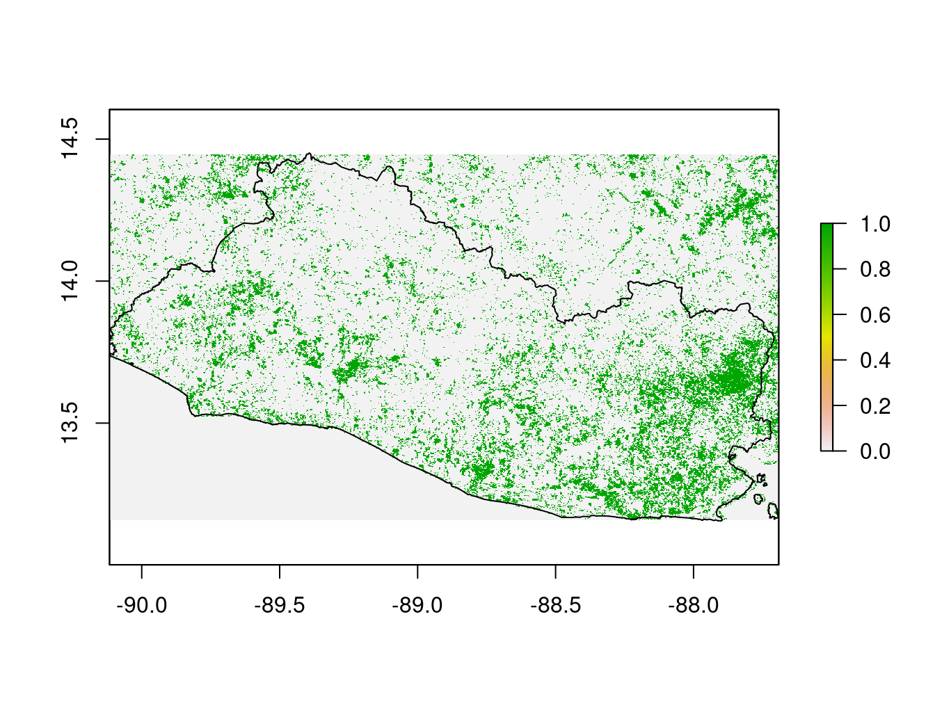
Figure 9.8: Soil Degradation, SDG indicator 15.3
9.5.5 Temperature
Next, we calculate the median and standard deviation of the temperature variations for the year 2017.
temp_median=raster::calc(temp_months,
fun = median,
na.rm = T)
temp_summaries=raster::stack(temp_median)
names(temp_summaries)=c("temp_median")
raster::plot(temp_median)
sp::plot(SLV_adm0,
add=T)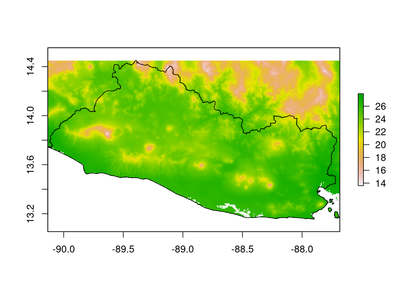
9.6 Distance Calculation
Distance to public services and businesses may be a good indicator of poverty and other development indicators: remote areas tend to be poorer and have lower levels of literacy. Furthermore, the distance to some natural features, such as the distance to the coast or the distance to forested areas, may be correlated with local economic development.
We compute below the distance to:
- Public services
- Hospitals (source: IDB)
- Health centers (source: IDB)
- Private, public, and other schools (source: IDB)
- Government offices (education and health excluded) (source: OSM)
- Any of the above
- Businesses
- Banks or ATMs (source: OSM)
- Any businesses, Bank or ATM included (source: OSM)
- Natural features
- Water bodies (land class from ESA)
- Cropland (land class from ESA)
- Forested areas (land class from ESA)
- Urban areas (land class from ESA)
9.6.1 Distance to Public Services
The first step is to create a raster to use as a canvas to compute distances. The distances will be computed from each raster cell’s center to the closest point of interest (e.g., the closest school). To have relatively good precision with the distance estimates, we will create a raster with a resolution of 100 meters. Note the use of the projected coordinates system from the segmento_sh shapefile.
# Create a raster for the computation of distances
raster_dist=raster::raster(raster::extent(segmento_sh),
crs=segmento_sh@proj4string,
res=c(100,100))
print(segmento_sh@proj4string)## CRS arguments:
## +proj=lcc +lat_0=13.783333 +lon_0=-89 +lat_1=13.316666 +lat_2=14.25
## +x_0=500000 +y_0=295809.184 +k_0=0.99996704 +datum=NAD27 +units=m
## +no_defsWe transform the CRS of the hospitals_sp shapefile to the corresponding projected CRS:
# Project the hospital shapefile ####
hospitals_proj=sp::spTransform(hospitals_sp,
segmento_sh@proj4string)We can now compute the distance from each cell center of the raster, raster_dist, to the projected shapefile of hospitals, hospitals_proj, with the function raster::distanceFromPoints.10
The distance map is plotted for inspection.
The color scale indicates the distance to hospitals.
The same process can be repeated for the other public services (not shown).
For the OSM data, two additional steps are required:
- The data is filtered to select only the public amenities defined as:
- Townhall
- Post office
- Courthouse
- Police station
- Prison
- Fire station
- Community center
- Public building (a loose OSM definition)
- The polygon data is rasterized to allow for distance calculation with the function
raster::distance- A buffer of 25 meters needs to be included as the function
raster::rasterizeconsiders a polygon to cross a cell only if it covers the cell center - The function
raster::distancecomputes the distance from all pixels with anNAvalue to the nearest pixel that is notNA.
- A buffer of 25 meters needs to be included as the function
# Distance to public amenities (health and education excluded) ####
amenities=c("townhall","post_office","courthouse","police",
"prison","public_building","fire_station","community_centre")
# Polygons
poi_poly_pubserv=as(subset(poi_poly_sh,
amenity%in%amenities),
"SpatialPolygons")
poi_poly_pubserv_proj=sp::spTransform(poi_poly_pubserv,
segmento_sh@proj4string)
poi_poly_pubserv_proj_buffer=rgeos::gBuffer(poi_poly_pubserv_proj,width=50)
poly_pubserv_proj_r=raster::rasterize(poi_poly_pubserv_proj_buffer, y=raster_dist)
dist2poly_pubserv=raster::distance(poly_pubserv_proj_r)
# Points
poi_points_pubserv=as(subset(poi_points_sh,
amenity%in%amenities),
"SpatialPoints")
poi_points_pubserv_proj=sp::spTransform(poi_points_pubserv,
segmento_sh@proj4string)
dist2points_pubserv=raster::distanceFromPoints(raster_dist,
poi_points_pubserv_proj)
dist2pubamen=min(dist2points_pubserv,
dist2poly_pubserv)Lastly, we compute the distance to any public services for each pixel by taking the minimum distance of the four distance maps:
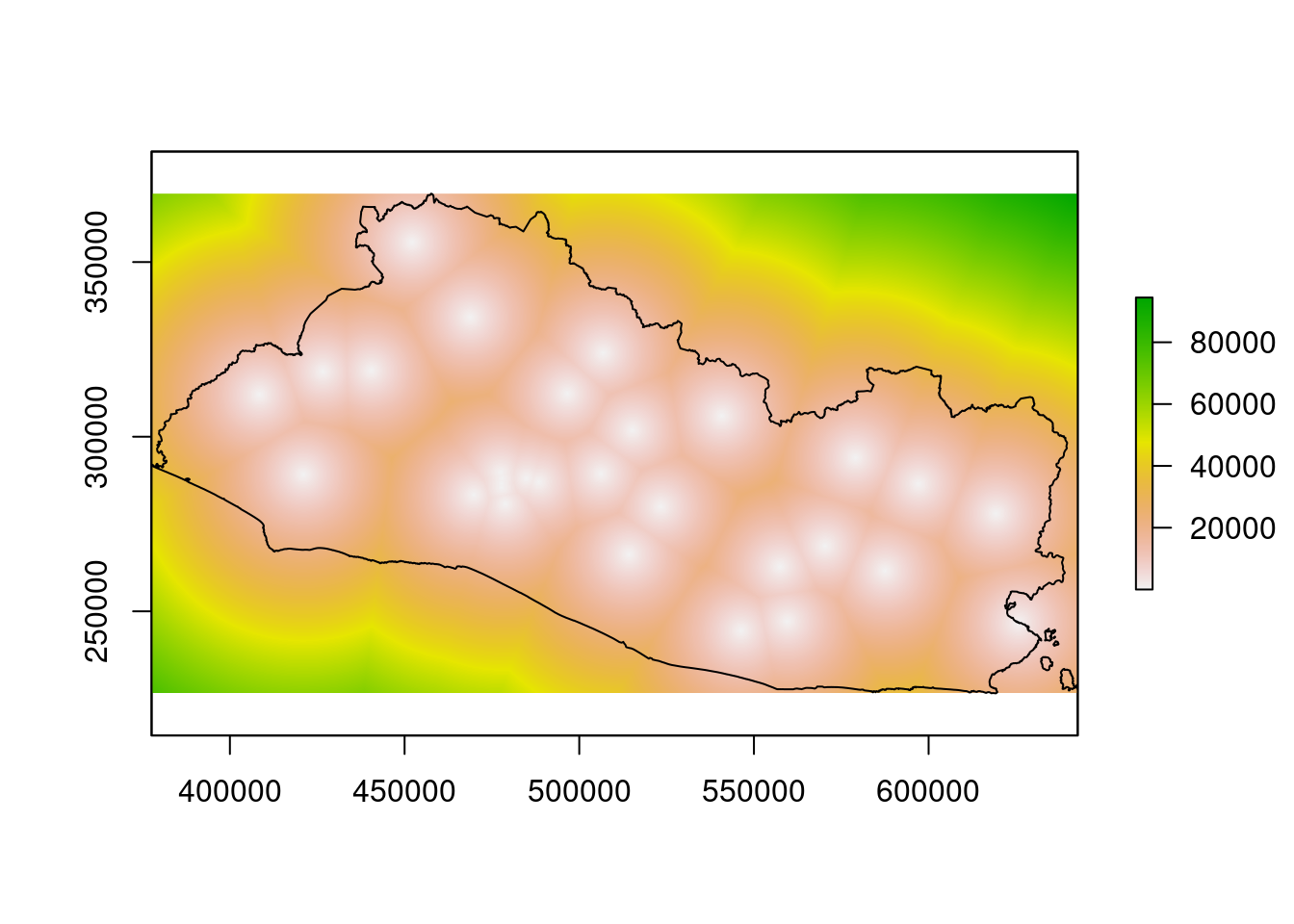
9.6.2 Distance to Businesses
The same approach is adopted for the distance to businesses. We start with the distance to financial-services access points, defined as banks and ATMs.
# Distance to FAPS ####
amenities=c("bank","atm")
poi_poly_fin=as(subset(poi_poly_sh,
amenity%in%amenities),
"SpatialPolygons")
poi_poly_fin_proj=sp::spTransform(poi_poly_fin,
segmento_sh@proj4string)
poi_poly_fin_proj_buffer=rgeos::gBuffer(poi_poly_fin_proj,width=50)
poly_fin_proj_r=raster::rasterize(poi_poly_fin_proj_buffer,
y=raster_dist)
dist2poly_fin=raster::distance(poly_fin_proj_r)
poi_points_fin=as(subset(poi_points_sh,
amenity%in%amenities),
"SpatialPoints")
poi_points_fin_proj=sp::spTransform(poi_points_fin,
segmento_sh@proj4string)
dist2points_fin=raster::distanceFromPoints(raster_dist,
poi_points_fin_proj)
dist2fin=min(dist2points_fin,
dist2poly_fin)We proceed with the other businesses. These are the OpenStreetMap business categories considered in addition to banks and ATMs: * Market * Foodcourt * Restaurant * Fast food vendor * Cafe * Bar * Ice cream shop * Pharmacy * Internet cafe * Cinema * Fuel vendor
# Businesses in amenities
amenities=c("marketplace","pharmacy","restaurant","fast_food","cafe","bar","ice_cream","food_court",
"internet_cafe", "cinema","fuel","atm","bank")
# Poly
poi_poly_eco=as(subset(poi_poly_sh,
amenity%in%amenities),
"SpatialPolygons")
poi_poly_eco_proj=sp::spTransform(poi_poly_eco,
segmento_sh@proj4string)
poi_poly_eco_proj_buffer=rgeos::gBuffer(poi_poly_eco_proj,width=50)
poly_eco_proj_r=raster::rasterize(poi_poly_eco_proj_buffer,
y=raster_dist)
dist2poly_eco=raster::distance(poly_eco_proj_r)
# Points
poi_points_eco=as(subset(poi_points_sh,
amenity%in%amenities),
"SpatialPoints")
poi_points_eco_proj=sp::spTransform(poi_points_eco,
segmento_sh@proj4string)
dist2points_eco=raster::distanceFromPoints(raster_dist,
poi_points_eco_proj)In addition to being listed in the amenity field of the OSM data, shop locations are also tagged separately. Given that shops are businesses, they are accounted for in the distance calculations.
# Businesses as shop
# Poly
poi_poly_shop=as(subset(poi_poly_sh,
is.na(shop)==F),
"SpatialPolygons")
poi_poly_shop_proj=sp::spTransform(poi_poly_shop,
segmento_sh@proj4string)
poi_poly_shop_proj_buffer=rgeos::gBuffer(poi_poly_shop_proj,width=50)
poly_shop_proj_r=raster::rasterize(poi_poly_shop_proj_buffer,
y=raster_dist)
dist2poly_shop=raster::distance(poly_shop_proj_r)
# Points
poi_points_shop=as(subset(poi_points_sh,
is.na(shop)==F),
"SpatialPoints")
poi_points_shop_proj=sp::spTransform(poi_points_shop,
segmento_sh@proj4string)
dist2points_shop=raster::distanceFromPoints(raster_dist,
poi_points_shop_proj)Finally, we gather all business-specific distance maps into one general “Distance to businesses” map.
9.6.3 Distance to Natural Features
Next, we compute the distance to natural features such as the coastline, urban areas, forested areas, and croplands.
We start by cropping the world’s coastlines to El Salvador’s boundaries. Once this operation is complete, we project the map and create the necessary buffer.
## Warning in proj4string(x): CRS object has comment, which is lost in output
## Warning in proj4string(x): CRS object has comment, which is lost in outputcoastline_proj=sp::spTransform(coastline_c,
segmento_sh@proj4string)
coastline_proj_buffer=rgeos::gBuffer(coastline_proj,width=50)
coastline_proj_r=raster::rasterize(coastline_proj_buffer,
y=raster_dist)
dist2coast=raster::distance(coastline_proj_r)To determine the distance to the urban areas, forested areas, croplands, and water bodies, we use NA for pixels that are not urban, not tree covered, not cropland, or not water bodies, respectively. We then use the function raster::distance to compute the distance from each NA pixel to the closest non-NA pixel.
# Distance to urban area ####
lc_urban=lc
lc_urban=raster::calc(lc_urban,
fun=function(x) {ifelse(x==190,1,NA)})
lc_urban_proj=raster::projectRaster(lc_urban,
crs=segmento_sh@proj4string)## Warning in rgdal::rawTransform(projfrom, projto, nrow(xy), xy[, 1], xy[, : Using
## PROJ not WKT2 strings## Warning in rgdal::rawTransform(projection(obj), crs, nrow(xy), xy[, 1], : Using
## PROJ not WKT2 strings## Warning in rgdal::rawTransform(projto_int, projfrom, nrow(xy), xy[, 1], : Using
## PROJ not WKT2 stringsdist2urban=raster::distance(lc_urban_proj)
# Distance to forest ####
lc_tree=lc
lc_tree=raster::calc(lc_tree,
fun=function(x) {ifelse(x%in%c(50,60),1,NA)})
lc_tree_proj=raster::projectRaster(lc_tree,
crs=segmento_sh@proj4string)## Warning in rgdal::rawTransform(projfrom, projto, nrow(xy), xy[, 1], xy[, : Using
## PROJ not WKT2 strings## Warning in rgdal::rawTransform(projection(obj), crs, nrow(xy), xy[, 1], : Using
## PROJ not WKT2 strings## Warning in rgdal::rawTransform(projto_int, projfrom, nrow(xy), xy[, 1], : Using
## PROJ not WKT2 stringsdist2tree=raster::distance(lc_tree_proj)
# Distance to cropland ####
lc_crop=lc
lc_crop=raster::calc(lc_crop,
fun=function(x) {ifelse(x%in%c(10,20,30,40),1,NA)})
lc_crop_proj=raster::projectRaster(lc_crop,
crs=segmento_sh@proj4string)## Warning in rgdal::rawTransform(projfrom, projto, nrow(xy), xy[, 1], xy[, : Using
## PROJ not WKT2 strings## Warning in rgdal::rawTransform(projection(obj), crs, nrow(xy), xy[, 1], : Using
## PROJ not WKT2 strings## Warning in rgdal::rawTransform(projto_int, projfrom, nrow(xy), xy[, 1], : Using
## PROJ not WKT2 stringsdist2crop=raster::distance(lc_crop_proj)
# Distance to water ####
lc_water=lc
lc_water=raster::calc(lc_water,
fun=function(x) {ifelse(x%in%c(210),1,NA)})
lc_water_proj=raster::projectRaster(lc_water,
crs=segmento_sh@proj4string)## Warning in rgdal::rawTransform(projfrom, projto, nrow(xy), xy[, 1], xy[, : Using
## PROJ not WKT2 strings## Warning in rgdal::rawTransform(projection(obj), crs, nrow(xy), xy[, 1], : Using
## PROJ not WKT2 strings## Warning in rgdal::rawTransform(projto_int, projfrom, nrow(xy), xy[, 1], : Using
## PROJ not WKT2 strings9.6.4 Stack the Distance Maps and Inspect the Results
Once the function raster::resample aligns the rasters on extent and resolution, the distance maps are stacked with the function raster::stack.
dist2coast_r=raster::resample(dist2coast,
dist2fin)
dist2water_r=raster::resample(dist2water,
dist2fin)
dist2crop_r=raster::resample(dist2crop,
dist2fin)
dist2tree_r=raster::resample(dist2tree,
dist2fin)
dist2urban_r=raster::resample(dist2urban,
dist2fin)
dist_stack=raster::stack(dist2schools_priv,
# dist2schools_pub,
dist2schools,
dist2health,
dist2hosp,
dist2pubamen,
dist2allpubserv,
dist2biz,
dist2fin,
dist2coast_r,
dist2water_r,
dist2crop_r,
dist2tree_r,
dist2urban_r)
names(dist_stack)=c("dist2schools_priv",
# "dist2schools_pub",
"dist2schools",
"dist2health",
"dist2hosp",
"dist2pubamen",
"dist2allpubserv",
"dist2biz",
"dist2fin",
"dist2coast_r",
"dist2water_r",
"dist2crop_r",
"dist2tree_r",
"dist2urban_r")We can now examine the results. The next maps show the distances to financial-service access points, businesses, private schools, and public schools (only the code for distance to financial-service access points is shown).
SLV_adm0_proj=sp::spTransform(SLV_adm0,
segmento_sh@proj4string)
raster::plot(dist_stack$dist2fin, main="Distance to financial access points, source: OSM")
sp::plot(SLV_adm0_proj,add=T)
sp::plot(waterbodies_proj,col="blue",add=T)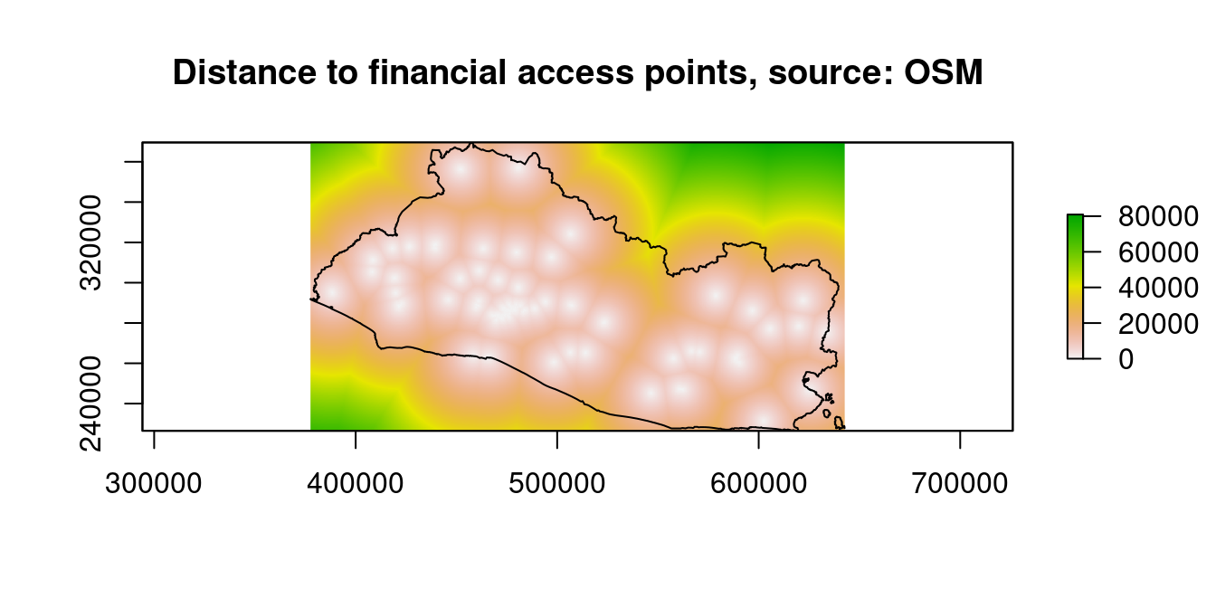
Figure 9.9: Distance to Financial Access Points
raster::plot(dist_stack$dist2biz, main="Distance to businesses, source: OSM")
sp::plot(SLV_adm0_proj,add=T)
sp::plot(waterbodies_proj,col="blue",add=T)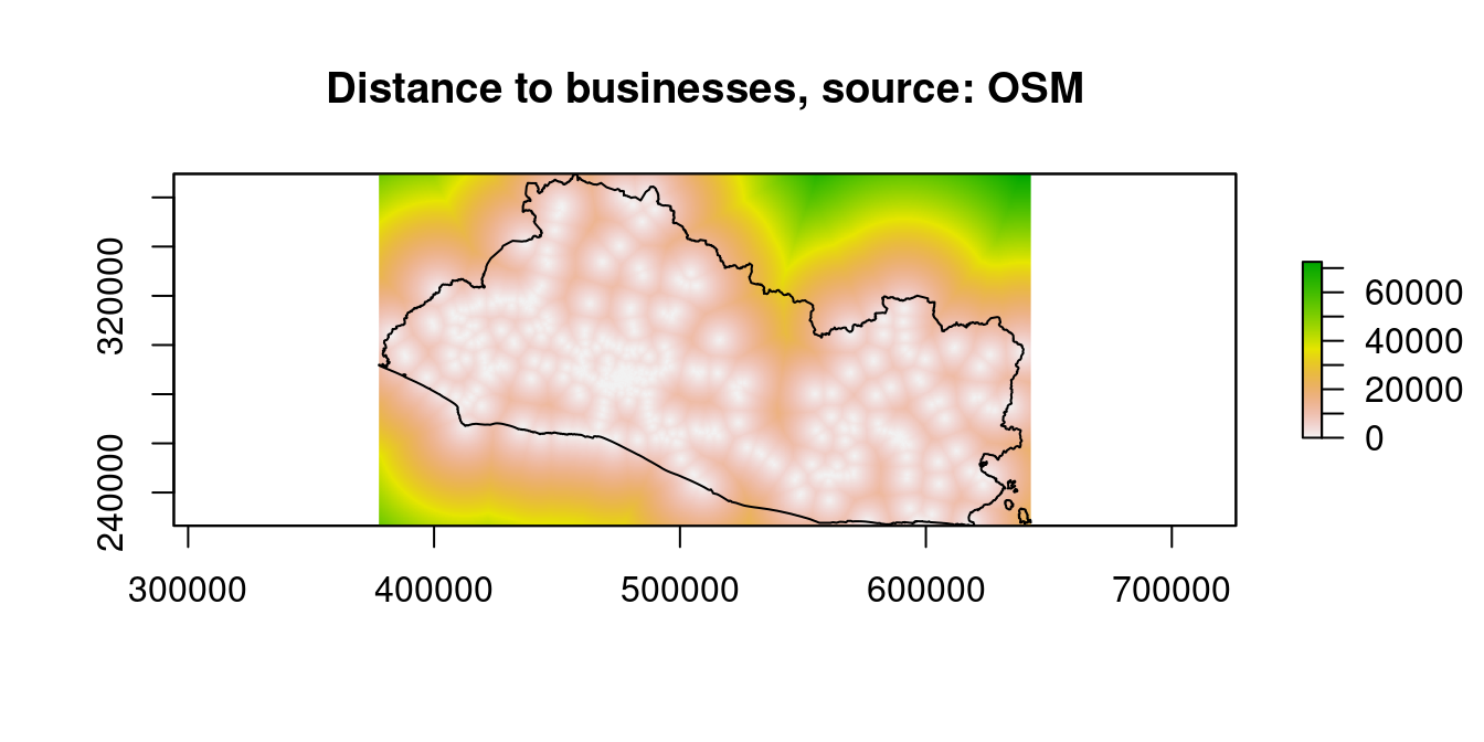
Figure 9.10: Distance to Financial Access Points
raster::plot(dist_stack$dist2schools_priv, main="Distance to private school, source: IDB")
sp::plot(SLV_adm0_proj,add=T)
sp::plot(waterbodies_proj,col="blue",add=T)
sp::plot(waterbodies_proj,col="blue",add=T)
# raster::plot(dist_stack$dist2schools_pub, main="Distance to public schools, source: IDB")
sp::plot(SLV_adm0_proj,add=T)
sp::plot(waterbodies_proj,col="blue",add=T)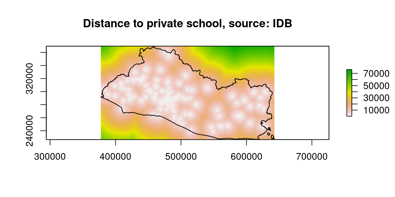
Figure 9.11: Distance to Financial Access Points
raster::plot(dist_stack$dist2urban_r, main="Distance to urban areas, source: IDB")
sp::plot(SLV_adm0_proj,add=T)
sp::plot(waterbodies_proj,col="blue",add=T)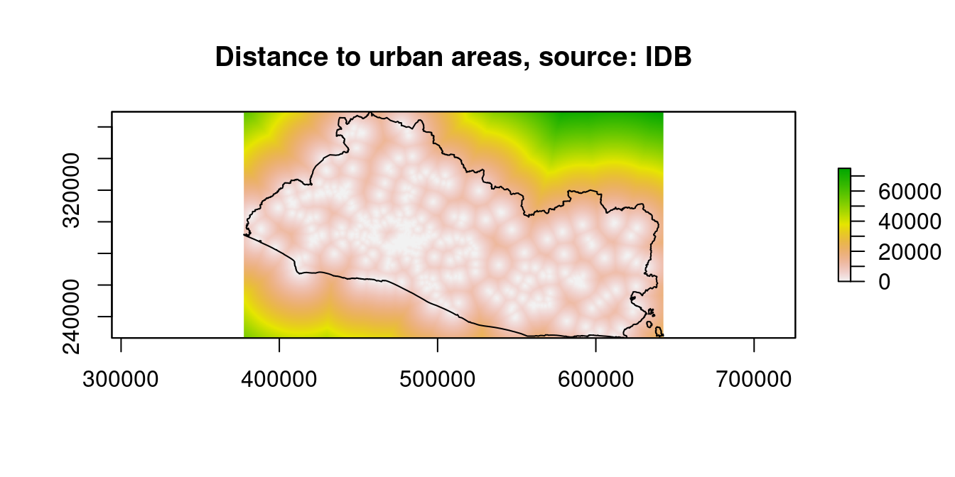
Figure 9.12: Distance to Financial Access Points
raster::plot(dist_stack$dist2hosp, main="Distance to hospital, source: IDB")
sp::plot(SLV_adm0_proj,add=T)
sp::plot(waterbodies_proj,col="blue",add=T)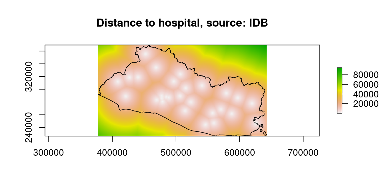
Figure 9.13: Distance to Financial Access Points
raster::plot(dist_stack$dist2pubamen, main="Distance to public amenities, source: OSM")
sp::plot(SLV_adm0_proj,add=T)
sp::plot(waterbodies_proj,col="blue",add=T)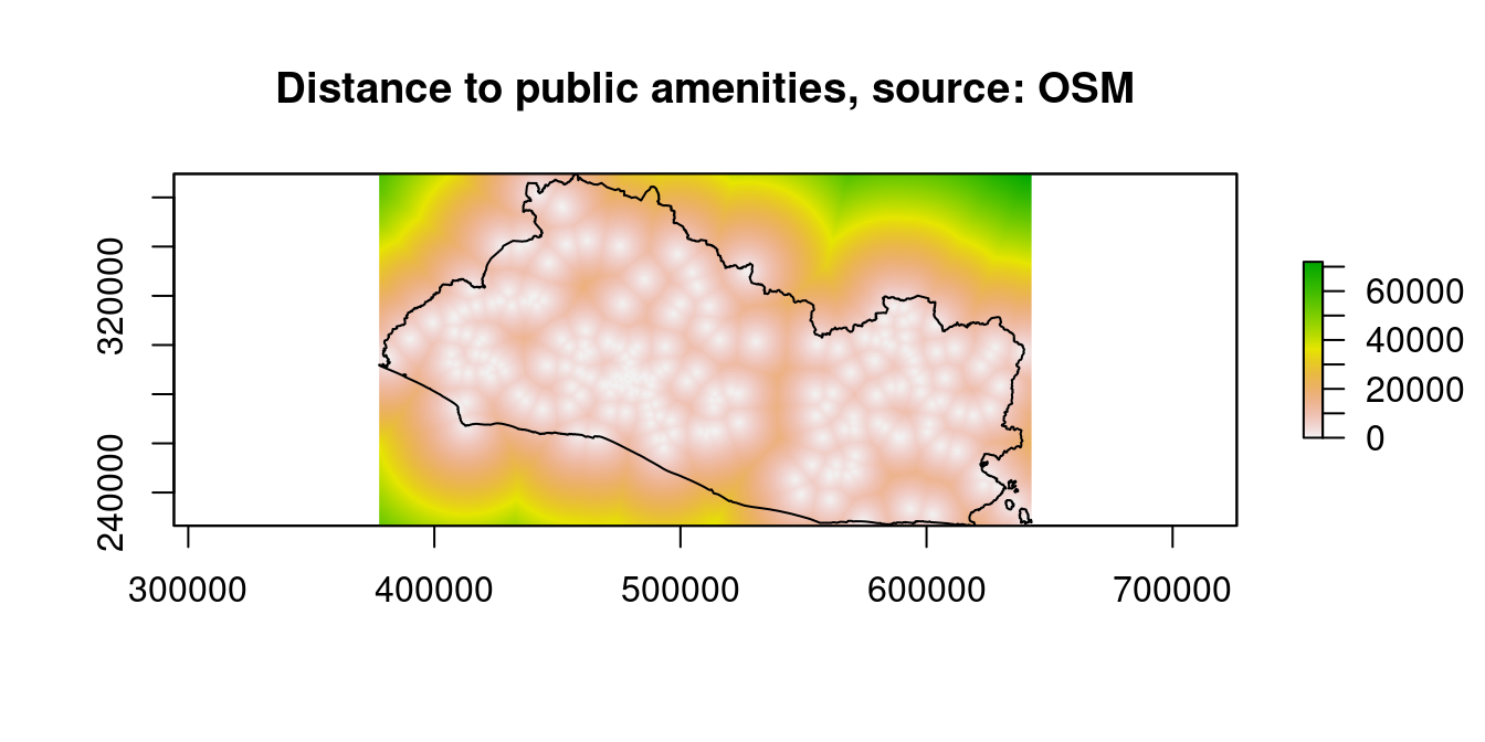
Figure 9.14: Distance to Financial Access Points
9.7 Spatial Statistics at the Segmento Level
The raster and vector layers built above need to be matched with the EHPM survey data for them to be used in the analysis. This can be done by either (1) identifying the centroid of each segmento and extracting the value of each covariate layer at the centroid of each segmento or (2) computing the spatial average, minimum, or maximum (or other) of each covariate for each segmento.
Although the first approach is simpler to implement, the second is preferred: data on poverty, income, and literacy are available at the segmento level because they are area data rather than point-referenced data. Therefore, it is best to provide spatial summary statistics at the same spatial-aggregation level rather than extracting data at the centroid of the segmento, which is an arbitrary location that might not be representative of the prevailing conditions in the segmento.
A prerequisite for merging data is to have all data defined by the same CRS.
9.7.1 Adjusting the CRS for Raster Extraction to Segmento
To make sure all the preprocessed RS layers are set to the same CRS, the following process is adopted: 1. Create a list of layers 2. Identify the layer with a different CRS 3. Re-project the layer with the different CRS
# Create the list of rasters
rasters_list=list(chirps_summaries,
soil_deg,soil_deg_SDG_index,
ndvi_17_summaries,ndvi_17_perc_summaries,
dem,
gpw_es,
temp_summaries,
dist2road,
dist2roadInter,
slope,
settlements,
dist2water,
lights_summaries,
lc,
dist_stack)
sum(unlist(lapply(rasters_list, raster::nlayers))) # Number of layers## [1] 34names(rasters_list)=c("chirps_summaries",
"soil_deg","soil_deg_SDG_index",
"ndvi_17_summaries","ndvi_17_perc_summaries",
"dem",
"gpw_es",
"temp_summaries",
"dist2road",
"dist2roadInter",
"slope",
"settlements",
"dist2water",
"lights_summaries",
"lc",
"dist_stack")
# Identify the rasters with a different projection
different_proj=which(lapply(rasters_list,
FUN=function(x) sp::proj4string(x)==sp::proj4string(segmento_sh_wgs))==F)
# Reproject these rasters to the same geographic coordinates system as the segmento
rasters_list[different_proj]=lapply(rasters_list[different_proj],
FUN=function(x) raster::projectRaster(x, crs=sp::proj4string(segmento_sh_wgs)))
# Turn the list items into object by replacing the original raster objects with
# he new raster objects with the correct coordinate system
for(i in 1:length(rasters_list)) {
assign(names(rasters_list)[i],
rasters_list[[i]])
}The same is done for the list of vector files (not shown), with the only difference being that the function raster::projectRaster is replaced by the function sp::spTransform because a vector is used.
9.7.2 Rasters
For each raster layer, we now need to get summary statistics for each segmento area. We will start by getting segmento area average value for each raster layer,11 except for the population, where we will also get the \(sum\), that is, total population count per segmento, and land class, where we will get the percentage of segmento area for a subset of classes.
The package velox rather than the standard extract function from the raster package is used, as it is much faster.12
rasters_extraction_list=c("chirps_summaries","soil_deg","soil_deg_SDG_index","ndvi_17_summaries","ndvi_17_perc_summaries",
"dem","temp_summaries","dist2road","dist2roadInter","slope","settlements","dist2water","lights_summaries","dist_stack")
seg_r_s=c() # Create an empty vector to store the extracted data
START_e=Sys.time() # Record the start time of the loop
for(r in rasters_extraction_list){ # Loop over the list of rasters
# Create a velox object from the raster
r_velox=velox::velox(get(r)) # The function `get(x)` interprets the character “x” as an
# object. In the code snippet below, it allows us to loop through the list of raster names.
ex.mat <- r_velox$extract(segmento_sh_wgs,
fun=function(x) mean(x,na.rm=T),
small=T) # Get the mean
seg_r_s=cbind(seg_r_s,ex.mat) # Add the extracted data as a new column
}## Warning in showSRID(uprojargs, format = "PROJ", multiline = "NO"): Discarded datum Unknown based on WGS84 ellipsoid in CRS definition,
## but +towgs84= values preserved
## Warning in showSRID(uprojargs, format = "PROJ", multiline = "NO"): Discarded datum Unknown based on WGS84 ellipsoid in CRS definition,
## but +towgs84= values preserved
## Warning in showSRID(uprojargs, format = "PROJ", multiline = "NO"): Discarded datum Unknown based on WGS84 ellipsoid in CRS definition,
## but +towgs84= values preserved
## Warning in showSRID(uprojargs, format = "PROJ", multiline = "NO"): Discarded datum Unknown based on WGS84 ellipsoid in CRS definition,
## but +towgs84= values preserved
## Warning in showSRID(uprojargs, format = "PROJ", multiline = "NO"): Discarded datum Unknown based on WGS84 ellipsoid in CRS definition,
## but +towgs84= values preserved
## Warning in showSRID(uprojargs, format = "PROJ", multiline = "NO"): Discarded datum Unknown based on WGS84 ellipsoid in CRS definition,
## but +towgs84= values preserved
## Warning in showSRID(uprojargs, format = "PROJ", multiline = "NO"): Discarded datum Unknown based on WGS84 ellipsoid in CRS definition,
## but +towgs84= values preserved
## Warning in showSRID(uprojargs, format = "PROJ", multiline = "NO"): Discarded datum Unknown based on WGS84 ellipsoid in CRS definition,
## but +towgs84= values preserved
## Warning in showSRID(uprojargs, format = "PROJ", multiline = "NO"): Discarded datum Unknown based on WGS84 ellipsoid in CRS definition,
## but +towgs84= values preserved
## Warning in showSRID(uprojargs, format = "PROJ", multiline = "NO"): Discarded datum Unknown based on WGS84 ellipsoid in CRS definition,
## but +towgs84= values preserved
## Warning in showSRID(uprojargs, format = "PROJ", multiline = "NO"): Discarded datum Unknown based on WGS84 ellipsoid in CRS definition,
## but +towgs84= values preserved
## Warning in showSRID(uprojargs, format = "PROJ", multiline = "NO"): Discarded datum Unknown based on WGS84 ellipsoid in CRS definition,
## but +towgs84= values preserved
## Warning in showSRID(uprojargs, format = "PROJ", multiline = "NO"): Discarded datum Unknown based on WGS84 ellipsoid in CRS definition,
## but +towgs84= values preserved
## Warning in showSRID(uprojargs, format = "PROJ", multiline = "NO"): Discarded datum Unknown based on WGS84 ellipsoid in CRS definition,
## but +towgs84= values preserved
## Warning in showSRID(uprojargs, format = "PROJ", multiline = "NO"): Discarded datum Unknown based on WGS84 ellipsoid in CRS definition,
## but +towgs84= values preserved
## Warning in showSRID(uprojargs, format = "PROJ", multiline = "NO"): Discarded datum Unknown based on WGS84 ellipsoid in CRS definition,
## but +towgs84= values preserved
## Warning in showSRID(uprojargs, format = "PROJ", multiline = "NO"): Discarded datum Unknown based on WGS84 ellipsoid in CRS definition,
## but +towgs84= values preserved
## Warning in showSRID(uprojargs, format = "PROJ", multiline = "NO"): Discarded datum Unknown based on WGS84 ellipsoid in CRS definition,
## but +towgs84= values preserved
## Warning in showSRID(uprojargs, format = "PROJ", multiline = "NO"): Discarded datum Unknown based on WGS84 ellipsoid in CRS definition,
## but +towgs84= values preserved
## Warning in showSRID(uprojargs, format = "PROJ", multiline = "NO"): Discarded datum Unknown based on WGS84 ellipsoid in CRS definition,
## but +towgs84= values preserved
## Warning in showSRID(uprojargs, format = "PROJ", multiline = "NO"): Discarded datum Unknown based on WGS84 ellipsoid in CRS definition,
## but +towgs84= values preserved
## Warning in showSRID(uprojargs, format = "PROJ", multiline = "NO"): Discarded datum Unknown based on WGS84 ellipsoid in CRS definition,
## but +towgs84= values preserved## Time difference of 2.950998 minscolnames(seg_r_s)=c(names(chirps_summaries),
names(soil_deg),
"soil_deg_SDG_index",
names(ndvi_17_summaries),
names(ndvi_17_perc_summaries),
"dem",names(temp_summaries),
"dist2road","dist2roadInter","slope","settlements","dist2water",
names(lights_summaries),
names(dist_stack))For the population raster, we get the \(sum\) per segment.
# Population
r_velox=velox::velox(gpw_es)
ex.mat_pop <- r_velox$extract(segmento_sh_wgs,
fun=function(x) sum(x,na.rm=T),
small=T) # get the sum
colnames(ex.mat_pop)="gpw_es_TOT"For land cover, we extract the share of each segmento area classified as
- Urban areas
- Land class: 190
- Land class: 190
- Tree-cover area13
- Land class: 50, tree cover broadleaved evergreen closed to open (>15 percent of pixel area)
- Land class: 60, tree cover broadleaved deciduous closed to open (>15 percent of pixel area)
- Cropland
- Land class: 10, cropland rainfed
- Land class: 20, cropland irrigated or post-flooding
- Land class: 30, mosaic cropland (>50 percent of pixel area)/natural vegetation (tree/shrub/ herbaceous cover) (<50 percent of pixel area)
- Land class: 40, mosaic natural vegetation (tree/shrub/herbaceous cover) (>50% of pixel area)/cropland (<50 percent of pixel area)
# Land class ####
r_velox=velox::velox(lc)
# Urban land class
ex.mat_urb <- r_velox$extract(segmento_sh_wgs,
fun=function(x) sum(x==190,na.rm=T)/(sum(x==190,na.rm=T)+sum(x!=190,na.rm=T)),
small=T) # Get the sum
# Tree cover
# 50;Tree cover broadleaved evergreen closed to open (>15%);0;100;0
# 60;Tree cover broadleaved deciduous closed to open (>15%);0;160;0
ex.mat_tree <- r_velox$extract(segmento_sh_wgs,
fun=function(x) sum(x%in%c(50,60, 100,110),na.rm=T)/(sum(x%in%c(50,60,100,110),na.rm=T)+sum(!(x%in%c(50,60,100,110)),na.rm=T)),
small=T) # Get the sum
# crop land
# 10;Cropland rainfed;255;255;100
# 20;Cropland irrigated or post-flooding;170;240;240
# 30;Mosaic cropland (>50%) / natural vegetation (tree shrub herbaceous cover) (<50%);220;240;100
# 40;Mosaic natural vegetation (tree shrub herbaceous cover) (>50%) / cropland (<50%) ;200;200;100
ex.mat_crop <- r_velox$extract(segmento_sh_wgs,
fun=function(x) sum(x%in%c(10,20,30,40),na.rm=T)/(sum(x%in%c(10,20,30,40),na.rm=T)+sum(!(x%in%c(10,20,30,40)),na.rm=T)),
small=T) # Get the sum
colnames(ex.mat_urb)="lc_urban"
colnames(ex.mat_tree)="lc_tree"
colnames(ex.mat_crop)="lc_crop"Lastly, the extracted data are added to a data frame before merging it with the segmento SpatialPolygonDataframe by binding its columns with the function cbind.
seg_r=cbind(seg_r_s,
ex.mat_pop,
ex.mat_urb,
ex.mat_tree,
ex.mat_crop) # Compile the extracted data
seg_r_df=as.data.frame(seg_r)
segmento_sh_wgs@data=cbind(segmento_sh_wgs@data,
seg_r_df)
# ogrDrivers()
# writeOGR(segmento_sh_wgs,
# paste0(dir_data,
# "spatial/shape/out/STPLAN_Segmentos_WGS84_wdata2.shp"),
# driver = "ESRI Shapefile",
# layer=1)
# 9.7.2.1 Quality Check
We now check that the extraction worked well and did not produce any missing values, which could be caused by the raster layers not providing any value for small segmentos on islands.
missing_r=apply(segmento_sh_wgs@data,2,FUN=function(x) which(is.na(x)))
missing_r=unique(c(unlist(missing_r)))
missing_SEG=segmento_sh_wgs%>%
subset(SEG_ID%in%segmento_sh_wgs$SEG_ID[missing_r])
missing_SEG_coords=sp::coordinates(missing_SEG)
leaflet(SLV_adm0)%>%
addPolygons()%>%
addMarkers(missing_SEG_coords[,1],missing_SEG_coords[,2])Figure 9.15: Observations with No Data
We observe in Figure 9.15 that most of the missing values are in border areas. Two main reasons explain these NA:
- A lot of raster maps produced by WorldPop and HDX used boundaries produced by the open source Global Administrative Boundaries project. Unfortunately, El Salvador’s boundaries in the GADM are incorrect.
- Most preprocessed rasters are clipped to not overpass the boundaries, coastline, and bodies of water. Thus, some small segmentos at the border, on the coast, or on the shore of Lago Ilopango are not covered.
To identify the raster with missing values, we used the code below.
missing_r=apply(segmento_sh_wgs@data,2,FUN=function(x) which(is.na(x)))
data.frame(n_miss=unlist(lapply(missing_r,length)),
var_miss=names(missing_r))%>%
arrange(desc(n_miss))%>%
filter(n_miss>0)## n_miss var_miss
## dist2road 23 dist2road
## dist2roadInter 23 dist2roadInter
## settlements 23 settlements
## temp_median 3 temp_median
## soil_carb 2 soil_carb
## soil_prod_prf 2 soil_prod_prf
## chirps_ev_2017 1 chirps_ev_2017
## chirps_ev_med 1 chirps_ev_med
## soil_luc 1 soil_luc
## soil_prod_state 1 soil_prod_state
## soil_prod_trj 1 soil_prod_trj
## soil_deg_SDG_index 1 soil_deg_SDG_index
## lc_urban 1 lc_urbanAs their number is relatively small (a max of 22 missing values for 13 covariates), we decided to simply replace the missing value with the cantonal average. For the one segmento where this did not work, we used the municipio average (code not shown).
9.7.3 Vectors
For the vectors, a choice has to be made on the type of statistics desired from each vector layer. Here are the spatial summary statistics we will compute:
- Livelihood Zone Map: the livelihood type of a segmento
- Schools: private and public schools, including the sum of each category and the total number
- Health facilities: hospitals and three categories of health centers, including the sum of each category and the sum of categories
- OpenStreetMap point of interests
- Buildings, including the total number
- Points of interest, including the total number
- Shops, including the total number
- Amenities, as classified into 12 categories, including the sums within the 12 categories and the total number
- OpenStreetMap roads, streets, or paths
- Length of roads, streets, or paths classified in nine categories and their sums
- Density of roads, streets, or paths classified in nine categories (length of roads/segmento area)
- Share of rural and urban roads in total roads, streets, or paths of the segmento
9.7.3.1 Livelihood Zones
As there is only one categorical value per area, the process is simple: the function over from the package sp is used to extract for each segmento the corresponding value of the “segmento_sh_wgs”’ SpatialPolygonDataFrame. The result of the function over is a data frame with one row per segmento of the segmento_sh_wgs. The livelihood zone code (“LZCODE”) and livelihood zone name (“LZNAMEEN”) are then added into the original data frame of segmento_sh_wgs.
# For each segment, extract the corresponding value of the segmento_sh_wgs's SpatialPolygonDataFrame
proj_WGS_84="+proj=longlat +datum=WGS84 +no_defs +ellps=WGS84 +towgs84=0,0,0"
segmento_sh_wgs=sp::spTransform(segmento_sh_wgs,
proj_WGS_84)## Warning in showSRID(uprojargs, format = "PROJ", multiline = "NO"): Discarded datum WGS_1984 in CRS definition,
## but +towgs84= values preserved## Warning in showSRID(uprojargs, format = "PROJ", multiline = "NO"): Discarded datum WGS_1984 in CRS definition,
## but +towgs84= values preservedLZ_seg=sp::over(segmento_sh_wgs,
LZ_sh)
LZ_seg=LZ_seg[,c("LZCODE","LZNAMEEN")]
# Add the livelihood zone data to segmento shape
segmento_sh_wgs@data$LZCODE=LZ_seg$LZCODE
segmento_sh_wgs@data$LZNAMEEN=LZ_seg$LZNAMEENCheck for any missing values.
## Mode FALSE TRUE
## logical 12421 14We see that 10 segmentos have no assigned livelihood zones. They are mapped in Figure 9.16.
missing_SEG=segmento_sh_wgs%>%
subset(SEG_ID%in%segmento_sh_wgs$SEG_ID[which(is.na(segmento_sh_wgs@data$LZNAMEEN))])
missing_SEG_coords=sp::coordinates(missing_SEG)
leaflet(SLV_adm0)%>%
addPolygons()%>%
addMarkers(missing_SEG_coords[,1],missing_SEG_coords[,2])Figure 9.16: Observations with No Data
All the missing values are in border areas: as the livelihood zone shapefile is not perfectly aligned to the segmento one, some segmentos fall outside the livelihood zone shapefile. A simple solution is to replace it manually after inspecting the map.
missing_canton=which(is.na(segmento_sh_wgs@data$LZNAMEEN)&
segmento_sh_wgs@data$CANTON%in%c("AREA URBANA","GUISQUIL"))
segmento_sh_wgs@data$LZNAMEEN[missing_canton]="Fishing, Aquaculture and Tourism Zone"
segmento_sh_wgs@data$LZCODE[missing_canton]="SV06"
missing_canton=which(is.na(segmento_sh_wgs@data$LZNAMEEN)&
segmento_sh_wgs@data$CANTON%in%c("ISLA ZACATILLO","ISLA MEANGUERITA"))
segmento_sh_wgs@data$LZNAMEEN[missing_canton]="Basic Grain and Labor Zone"
segmento_sh_wgs@data$LZCODE[missing_canton]="SV01"
missing_canton=which(is.na(segmento_sh_wgs@data$LZNAMEEN)&
segmento_sh_wgs@data$CANTON=="EL JOCOTILLO")
segmento_sh_wgs@data$LZNAMEEN[missing_canton]="Sugarcane, Agro-Industry and Labor Zone"
segmento_sh_wgs@data$LZCODE[missing_canton]="SV03"
summary(is.na(segmento_sh_wgs@data$LZNAMEEN))## Mode FALSE
## logical 12435## Mode FALSE
## logical 124359.7.3.2 Schools
The process of extracting the schools’ and health facilities’ data follows the same principle. The difference is that the data are point data instead of polygon data. The schools and health facilities datasets are the SpatialPointsDataFrame. The SpatialPointsDataFrame is first transformed into a SpatialPoints object using the function as. The function over is then run, with an additional parameter specified: fn=sum. This tells the function over to compute the sum of SpatialPoints per segmento, that is, the number of schools per segmento. For segmentos where there are no schools, the function over yields an NA value. NA values a replaced by zeros.
# Schools
# Total sum of schools
sch_seg=sp::over(segmento_sh_wgs,
as(school_sh, "SpatialPoints"),
fn=sum,na.rm=T)
# Replace the NA value
sch_seg[which(is.na(sch_seg))]=0The same process is done for public and private schools separately. The function subset is used to subset only one category.
# N public schools
sch_pub_seg=sp::over(segmento_sh_wgs,
as(subset(school_sh,
Sector!="PRIVADO"),
"SpatialPoints"),
fn=sum,na.rm=T)
sch_pub_seg[which(is.na(sch_pub_seg))]=0
# N private schools
sch_pri_seg=sp::over(segmento_sh_wgs,
as(subset(school_sh,
Sector=="PRIVADO"),
"SpatialPoints"),
fn=sum,na.rm=T)
sch_pri_seg[which(is.na(sch_pri_seg))]=0Lastly, the newly created covariates are added to the SpatialPolyongsDataFrame segmento_sh_wgs.
# Add the school data to segmento shape
segmento_sh_wgs@data$sch=sch_seg
segmento_sh_wgs@data$sch_pub=sch_pub_seg
segmento_sh_wgs@data$sch_pri=sch_pri_segThe process is repeated for health facilities before adding the covariate to segmento_sh_wgs (not shown).
9.7.3.3 OpenStreetMap Data
The OpenStreetMap data are provided in three sets of files:
- Buildings polygons (hotosm_slv_buildings_polygons.shp)
- Points-of-interest points (hotosm_slv_points_of_interest_points.shp)
- Points-of-interest polygons (hotosm_slv_points_of_interest_polygons.shp)
For the buildings data, the sum of buildings per segmento is computed. This indicates how urban a segmento is.
proj_WGS_84="+proj=longlat +datum=WGS84 +no_defs +ellps=WGS84 +towgs84=0,0,0"
buildings_poly_sh=sp::spTransform(buildings_poly_sh,
proj_WGS_84)## Warning in showSRID(uprojargs, format = "PROJ", multiline = "NO"): Discarded datum WGS_1984 in CRS definition,
## but +towgs84= values preservedbuild_seg=sp::over(segmento_sh_wgs,
as(buildings_poly_sh,
"SpatialPolygons"),
fn=sum,na.rm=T)
build_seg[which(is.na(build_seg))]=0
# Add the building data to segmento shape
segmento_sh_wgs@data$building=build_segFor the points of interest vectors (points and poly), the number of locations per segmento identified as a “shop” in OSM, that is, a place selling retail products or services, is calculated. This indicates how urban a segmento is and can shed some light on local economic dynamism.
proj_WGS_84="+proj=longlat +datum=WGS84 +no_defs +ellps=WGS84 +towgs84=0,0,0"
poi_poly_sh=sp::spTransform(poi_poly_sh,
proj_WGS_84)## Warning in showSRID(uprojargs, format = "PROJ", multiline = "NO"): Discarded datum WGS_1984 in CRS definition,
## but +towgs84= values preserved# Shop
shop_poly_seg=sp::over(segmento_sh_wgs,
as(subset(poi_poly_sh,
is.na(shop)==F),
"SpatialPolygons"),
fn=sum,na.rm=T)
shop_poly_seg[which(is.na(shop_poly_seg))]=0
shop_points_seg=sp::over(segmento_sh_wgs,
as(subset(poi_points_sh,
is.na(shop)==F),
"SpatialPoints"),
fn=sum,na.rm=T)
shop_points_seg[which(is.na(shop_points_seg))]=0
shop_n=shop_points_seg+shop_poly_seg
# Add the shop data to segmento shape
segmento_sh_wgs@data$shop=shop_nNext, the number of amenities according to 11 categories is computed.
## Warning in kableExtra::column_spec(., 3, width = "7cm"): Please specify format
## in kable. kableExtra can customize either HTML or LaTeX outputs. See https://
## haozhu233.github.io/kableExtra/ for details.| Category | Feature’s name in the data | OSM amenity categories |
|---|---|---|
| Financial access points | fin | bank, atm |
| Marketplace | mkt | marketplace |
| Bus Station | bus | bus_station |
| Parking | parking | parking |
| Place of Worship | worship | place_of_worship |
| Health service | health_srv | pharmacy, clinic, dentist, doctor, hospital |
| Food and drink | food | restaurant, fast_food, cafe, bar, ice_cream, food_court |
| Culture and Education | cult_educ | school, college, university, community_centre, theatre, arts_centre, internet_cafe, cinema |
| Fuel: Petrol station | fuel | fuel |
| Official buildings | official | townhall, post_office, courthouse, police, prison, public_building, fire_station |
The for loop below executes the extraction.
for(i in 1: length(list_amenities)){
extracted_poly_seg=sp::over(segmento_sh_wgs,
as(subset(poi_poly_sh,
amenity%in%list_amenities[[i]]),
"SpatialPolygons"),
fn=sum,na.rm=T)
extracted_poly_seg[which(is.na(extracted_poly_seg))]=0
extracted_point_seg=sp::over(segmento_sh_wgs,
as(subset(poi_points_sh,
amenity%in%list_amenities[[i]]),
"SpatialPoints"),
fn=sum,na.rm=T)
extracted_point_seg[which(is.na(extracted_point_seg))]=0
extracted_seg=extracted_point_seg+extracted_poly_seg
assign(list_amenities_name[[i]],
extracted_seg)
}
# Add the shop data to segmento shape
unlist(list_amenities_name)## [1] "fin" "mkt" "bus" "parking" "worship"
## [6] "health_srv" "food" "cult_educ" "fuel" "official"segmento_sh_wgs@data$fin=fin
segmento_sh_wgs@data$mkt=mkt
segmento_sh_wgs@data$bus=bus
segmento_sh_wgs@data$parking=parking
segmento_sh_wgs@data$worship=worship
segmento_sh_wgs@data$health_srv=health_srv
segmento_sh_wgs@data$food=food
segmento_sh_wgs@data$cult_educ=cult_educ
segmento_sh_wgs@data$fuel=fuel
segmento_sh_wgs@data$official=officialLastly, a series of covariates is computed on the roads data. As the goal is to measure length, the first step is to change the CRS of the roads vector into a projected coordinates system with units expressed in meters. The CRS of the original segmento data is used.
## Warning in sp::proj4string(segmento_sh): CRS object has comment, which is lost
## in outputThe OSM ‘roads’ are then regrouped into nine categories according to their highway class.
## Warning in kableExtra::column_spec(., 3, width = "7cm"): Please specify format
## in kable. kableExtra can customize either HTML or LaTeX outputs. See https://
## haozhu233.github.io/kableExtra/ for details.| Category | Feature’s name | OSM highway class |
|---|---|---|
| Fast track | fast_track | motorway_link, motorway, trunk_link, trunk, primary_link, primary |
| Secondary | secondary | secondary, secondary_link |
| Tertiary | tertiary | tertiary_link, tertiary |
| Residential | residential | residential, corridor |
| Rural track | rural_track | track |
| Pedestrian and bike line | urban_no_motor | living_street, cycleway, steps, path, footway, pedestrian, service |
| Bus lane | bus | bus_stop, bus_guideway |
| Luxury | luxury | raceway, bridleway |
| Unclassified | unclassified | no construction, unclassified, road |
The length of roads’ segments per segmento and according to the roads’ categories is computed using the function lineLength applied via over. The results are expressed in meters, as the unit of the CRS is meters.
# Length of roads
proj_WGS_84="+proj=longlat +datum=WGS84 +no_defs +ellps=WGS84 +towgs84=0,0,0"
segmento_sh=sp::spTransform(segmento_sh,
proj_WGS_84)## Warning in showSRID(uprojargs, format = "PROJ", multiline = "NO"): Discarded datum WGS_1984 in CRS definition,
## but +towgs84= values preserved## Warning in showSRID(uprojargs, format = "PROJ", multiline = "NO"): Discarded datum WGS_1984 in CRS definition,
## but +towgs84= values preservedlength_all_seg=sp::over(segmento_sh,
as(roads_lines_pr,
"SpatialLines"),
fn=lineLength,
na.rm=T)
length_all_seg[is.na(length_all_seg)]=0
for(i in 1:length(list_road_types)){
roads_type_sub=subset(roads_lines_pr,
highway %in% list_road_types[[i]])
length_seg=sp::over(segmento_sh,
as(roads_type_sub,
"SpatialLines"),
fn=lineLength,
na.rm=T)
length_seg[is.na(length_seg)]=0
assign(list_road_names[[i]],
length_seg)
}
# Add the road length data to the shapefile
segmento_sh_wgs@data$all_roads=length_all_seg
segmento_sh_wgs@data$fast_track=fast_track
segmento_sh_wgs@data$secondary=secondary
segmento_sh_wgs@data$tertiary=tertiary
segmento_sh_wgs@data$residential=residential
segmento_sh_wgs@data$rural_track=rural_track
segmento_sh_wgs@data$urban_no_motor=urban_no_motor
segmento_sh_wgs@data$bus=bus
segmento_sh_wgs@data$luxury=luxury
segmento_sh_wgs@data$unclassified=unclassified9.7.3.4 Normalizing the Road Data
The road network is normalized by the area of segmento: we obtain the kilometers of roads per square kilometer. The density of roads is computed as the length of roads divided by the area of segmento. The latter is already computed in the shapefile and stored in the feature Shape_Area.
# Density: length km/area
road_density_all=length_all_seg/segmento_sh@data$Shape_Area
for(i in 1:length(list_road_types)){
density_type_i=get(list_road_names[[i]])/segmento_sh_wgs@data$Shape_Area
assign(paste0("dens_",
list_road_names[[i]]),
density_type_i)
}
# Add the road density data to the shapefile
segmento_sh_wgs@data$dens_all_roads=road_density_all
segmento_sh_wgs@data$dens_fast_track=dens_fast_track
segmento_sh_wgs@data$dens_secondary=dens_secondary
segmento_sh_wgs@data$dens_tertiary=dens_tertiary
segmento_sh_wgs@data$dens_residential=dens_residential
segmento_sh_wgs@data$dens_rural_track=dens_rural_track
segmento_sh_wgs@data$dens_urban_no_motor=dens_urban_no_motor
segmento_sh_wgs@data$dens_bus=dens_bus
segmento_sh_wgs@data$dens_luxury=dens_luxury
segmento_sh_wgs@data$dens_unclassified=dens_unclassified9.8 Merging the Covariates with the EHPM Data
The data from SpatialPolygonDataframe are saved to a standard data frame.
Once the EHPM survey data tables/ehpm-2017.csv are loaded, select only the development indicators and the household id “idboleta.” The idboleta is used to match the EHPM with the segmento ID in tables/Identificador de segmento.xlsx. Lastly, the SEG_ID is used to match the survey data with the predictor.
# Save the data stored in segmento_sh_wgs@data in a standard data frame
# Select a subset of the covariates
predictors=segmento_sh_wgs@data
# Survey data
ehpm17=read.csv(paste0(dir_data,
"tables/ehpm-2017.csv"))
# Read the files with the segmento ID and the idboleta
segID=readxl::read_xlsx(paste0(dir_data,
"tables/Identificador de segmento.xlsx"),
sheet="2017")
# Select only the development indicators
ehpm17_dev_indic=ehpm17%>%
dplyr::select(municauto,
idboleta,
pobreza, # Poverty
ingpe, # Household income
r202a, # Sabe leer y escribir (knows how t oread and write)
r106 # Age
) %>%
dplyr::rename("lit"="r202a", # Rename these 2 variables
"age"="r106")%>%
dplyr::mutate(over_15=ifelse(age>=15,1,0),
literate=ifelse(lit==1,1,0),
literate_over_15=over_15*literate) # Literate and over 15 years old
# Match the survey data with the segID
ehpm17_seg=ehpm17_dev_indic%>%
left_join(segID,
by="idboleta")%>%
rename("SEG_ID"="seg_id")Below, we filter out all the survey participants who are less than 16 years old and compute development indicators for the population that is 16 years of age and above.
# Aggregate the survey data at the segmento level
ehpm17_seg_agg=ehpm17_seg%>%
filter(over_15==1)%>%
group_by(SEG_ID)%>%
summarise(municauto=unique(municauto),
n_obs=n(),
pobreza_extrema=sum(pobreza==1,na.rm = T)/n(),
pobreza_mod=sum(pobreza%in%c(1,2),na.rm = T)/n(),
literacy_rate=sum(literate_over_15,na.rm = T)/n(),
ingpe=median(ingpe,na.rm = T))## `summarise()` ungrouping output (override with `.groups` argument)# Merge the aggregated survey data with the predictor data
ehpm17_predictors=ehpm17_seg_agg%>%
right_join(predictors%>%
mutate(SEG_ID=as.character(SEG_ID)),
by="SEG_ID")# Write out the file
write.csv(ehpm17_predictors,
paste0(dir_data,
"out/ehpm17_predictors2.csv"),
row.names = F)## [1] "80 predictors"The .csv file out/ehpm17_predictors.csv contains the 79 predictors derived above plus the following development indicators:
## Warning in kableExtra::column_spec(., 3, width = "7cm"): Please specify format
## in kable. kableExtra can customize either HTML or LaTeX outputs. See https://
## haozhu233.github.io/kableExtra/ for details.| Variable name | Definition |
|---|---|
| pobreza_extrema | Proportion of individuals 15 years in extreme poverty: income below |
| pobreza_mod | Proportion of individuals 15 years in moderate poverty: income below $107.26 in urban areas or $66.90 in rural areas |
| literacy_rate | Proportion of individuals 15 years or older who can read and write |
| ingpe | Median income of individuals 15 years or older (USD) |
9.9 Summary
The process of going from raw RS layers to a SpatialPolygonDataframe ready for analysis can be summarized as follows:
- Load the RS layers.
- Create summaries for the RS layers that come with a time dimension (e.g., average precipitation over the last 30 years).
- Perform additional raster calculation as required (e.g., compute the Soil degradation index based on a soil degradation sub-indicator).
- Compute the distance metrics to public services, businesses, and some natural features.
- Align the CRSs across layers (geographic or projected).
- Aggregate the RS layers to the map of interest (e.g., the segmento map) with a chosen set of spatial statistics.
- Match the RS aggregates with the outcome data (poverty, income, literacy).
- Write the data frame to a
.csvfile for later use.
The 22 main data sources are summarized in the SpatialPolygonDataframe “segmento_sh_wgs” into 79 segmento-level spatial statistics listed on the next table. These are the candidate covariates to predict average income, poverty, and literacy measured in the 2017 EHPM survey.
## Warning in kableExtra::column_spec(., 3, width = "7cm"): Please specify format
## in kable. kableExtra can customize either HTML or LaTeX outputs. See https://
## haozhu233.github.io/kableExtra/ for details.| Category | Features |
|---|---|
| Precipitation | chirps_ev_2017, chirps_ev_med |
| Soil degradation | soil_carb, soil_luc, soil_prod_state, soil_prod_prf, soil_prod_trj, soil_deg_SDG_index |
| Vegetation Greenness (NDVI) | ndvi_17_median, ndvi_17_sd, ndvi_17_sum, ndvi_17_perc_median, ndvi_17_perc_sd, ndvi_17_perc_sum |
| Altitude (DEM) | dem |
| Population density | gpw_es, pop_dens, gpw_es_TOT |
| Temperature | temp_median |
| Livelihood Zones | LZCODE,LZNAMEEN |
| Education | dist2schools_priv, dist2schools_pub,dist2schools |
| Health services | dist2health, dist2hosp |
| Buildings | people_building |
| Shops | See distances |
| Other points of interest | See distances |
| Roads | dens_all_roads, dens_fast_track, dens_secondary, dens_tertiary, dens_residential, dens_rural_track, dens_urban_no_motor, dens_bus, dens_luxury, dens_unclassified |
| Slope | slope |
| Distances | dist2road, dist2roadInter, dist2water |
| Lights at night | lights_mean, lights_sd |
| Land Classes | lc_urban,lc_crop,lc_tree |
| Distance | dist2schools_priv, dist2schools_pub, dist2schools, dist2health, dist2hosp, dist2pubamen, dist2allpubserv, dist2biz, dist2fin, dist2coast_r, dist2water_r, dist2crop_r, dist2tree_r, dist2urban_r |
References
Fick, S. E., and R. J. Hijmans. 2017. “WorldClim 2: New 1-Km Spatial Resolution Climate Surfaces for Global Land Areas.” International Journal of Climatology 37 (12): 4302–15.
Henderson, Storeygard, J. V., and D. N. Weil. 2012. “Measuring Economic Growth from Outer Space.” American Economic Review 102 (2): 994–1028.
http://desktop.arcgis.com/en/arcmap/10.3/guide-books/map-projections/about-geographic-coordinate-systems.htm↩︎
http://desktop.arcgis.com/en/arcmap/10.3/guide-books/map-projections/about-projected-coordinate-systems.htm↩︎
Plotting these data allowed us in the first instance to identify the error in the naming of the coordinates: latitudes are actually longitudes and vice-versa. We therefore needed to use the
renamecommand.↩︎“A RasterBrick is a multilayer raster object that is typically created from a multilayer (band) file, but it can also exist entirely in memory. It is similar to a RasterStack (that can be created with stack), but processing time should be shorter when using a RasterBrick. Yet, RasterBricks are less flexible, as they can point only to a single file” (Hijmans 2019b).↩︎
TRENDS.EARTH (formerly the Land Degradation Monitoring Toolbox) is a QGIS plugin tool used to monitor land changes, including changes in productivity, land cover, and soil organic carbon. The tool supports land degradation monitoring for reporting to the Global Environment Facility (GEF) and United Nations Convention to Combat Desertification (UNCCD). Furthermore, it is used to track the progress toward the achievement of SDG Target 15.3, Land Degradation Neutrality (LDN).↩︎
The function
raster::distanceFromPointsis not very efficient and takes a few seconds to run. In countries with larger territories, and hence larger data volumes, running GRASS from R via ‘rgrass7’ is the way to go.↩︎Other spatial summaries could be investigated (e.g., average, median, minimum, maximum, standard deviation, sum, etc.); however, we focus on the mean for the sake of expediency.↩︎
The process took about 2 minutes and 30 seconds with
velox, while it did not complete withraster::extractafter 2 hours on 16GB RAM PC operating under Windows 10 on an Intel(R) Core(TM) i7-7700 HQ CPU @2.8 GHz. “Velox is fast because all raster computations are performed in C++ (using the excellent Rcpp API), and all data is held in memory”(Hunziker 2017).↩︎We focus on classes 50 and 60, as those are the most common.↩︎