Section 3 Data exploration and preselection of covariates
The data used in the model can be separated into two main categories:
- The outcome variables, which are the three development indicators (income, poverty, and literacy)
- The covariates, which are the set of predictors derived in Section 9 that will be used to predict the outcome variables in segmentos not sampled in the EHPM survey.
When exploring the outcome data, the aim is to identify possible issues such as a lack of variation or the presence of outliers. The exploration also helps in specifying the likelihood function for the outcome data (e.g., Gaussian, gamma, beta, etc.).
For the covariates, we start by reducing their number to limit the effect of multicollinearity, which is the presence of highly correlated covariates in the model. Reducing the number of covariates will also reduce the risk of retaining covariates because of chance correlation in a next stepwise covariates selection process as shown in section 5.
Lastly, we will investigate the correlation of the preselected covariates with the outcome variables.
3.1 Outcome Variables: Distribution and Outliers
3.1.1 Income
We start by exploring the distribution of the median income per segmento. It is named ingpe in the dataset:
Figure 3.1: Median income per segmento
As is common with income distributions, this distribution is right skewed: the median income is between USD 95 and 105 in most segmentos and reaches values above USD 200 in a few of them. An option is to log-transform the data to make it Gaussian.1 Another option is to model income with a gamma likelihood function, which accounts for the asymmetry of the income distribution.
Figure 3.2: Median Income Map
Figure 3.2 shows that all the segmentos with a median income above USD 265 (blue markers) are clustered together in urban centers, while the four with an income above USD 700 (gold markers) are located in Antiguo Cuscatlan, one of the country’s wealthiest neighborhoods where several embassies are located.
The national statistical office of El Salvador (DIGESTYC) classifies segmentos into rural and urban. Figure 3.3 shows the log-transformed distribution of median income for rural and urban segmentos separately.
Figure 3.3: Rural-Urban Median Income Distribution
Figure 3.3 shows that log transformation appears to be successful at making the distribution Gaussian. As seen in Figure 3.2, the median income is higher among urban than rural segmentos.
Furthermore, the main difference between the rural and urban income distributions is a location shift: the variance or skewness of the income distribution does not appear to vary significantly between rural and urban segmentos. Figure 3.3 suggests that a single model could be used provided that a binary covariate identifying rural and urban segmentos is used in the model (instead of running separate models for rural and urban segmentos).
In summary, this first exploration of the median income outcome data suggests that one could use either a gamma or a Gaussian likelihood function. In the latter case, income should be log-transformed. Furthermore, there are clear spatial patterns whereby urban areas have higher income levels than rural ones and segmentos that are close to each other tend to have similar income levels. Explicitly modeling spatial dependency is hence likely to improve the model’s goodness of fit. Lastly, we do not see any major difference between the distributions of income of rural and urban segmentos except for a location shift (all values shifted to the right among urban segmentos). A single model run both on rural and urban segmentos appears appropriate provided that a binary covariate identifying the rural or urban category is used.
3.1.2 Literacy
The variable literacy_rate provides the proportion of survey participants 16 years or older who can read and write. Its domain is bounded between 0 percent to 100 percent.
Figure 3.4: Rural-Urban Literacy Rates
The distribution of literacy in rural and urban segmentos appears quite different. Of the 950 urban segmentos, 181 have a 100 percent literacy rate among adult EHPM respondents. In contrast, no such spike is observed in the rural areas. This finding suggests that literacy could be modeled as a two-step process for urban areas: (1) the presence/absence of illiteracy is modeled, and (2) the proportion of illiteracy is modeled. In rural areas, only the second step would be necessary.
Figure next figure shows the map of literacy for the EHPM segmentos.
Figure 3.5: Literacy Rate Map
There is a clear spatial pattern: literacy rates are highest in urban areas, particularly around the capital city. Areas in the northwest (the departments of San Miguel, Morazan, and La Union) have low literacy levels.
In summary, modeling literacy will be more complex than modeling income. First, a zero-inflated model might be appropriate, particularly for urban segmentos. Second, the distribution of literacy appears to vary between rural and urban segmentos, and not only in terms of the location. Therefore, separate or mixed models for rural and urban segmentos might be more appropriate. In both cases, a beta likelihood function might be appropriate, as literacy rates are bounded between 0 and 100 percent. Lastly, there is a clear spatial pattern suggesting that explicitly taking the spatial dependence structure into account will increase the model’s goodness of fit.
3.1.3 Moderate Poverty
The variable pobreza_mod provides the proportion of survey participants 16 years or older living in moderate poverty. Its domain is bounded between 0 to 1.
Figure 3.6: Rural-Urban Moderate Poverty Rate
Figure 3.6 shows that more than 100 urban segmentos have no adult EHPM respondents living in poverty but no rural segmento does. Except for this important difference, the distribution of poverty of rural and urban segmentos does not appear to differ much.
Figure 3.7 shows the map of moderate poverty for the EHPM segmentos.Figure 3.7: Moderate Poverty Map
Interestingly, the picture is much less clear when mapping moderate poverty than income. However, the general urban-rural divide appears to hold.
As poverty is measured as a proportion, we will use a beta likelihood. Given the high number of segmentos with zero respondents living in poverty, we will test a zero-inflated beta likelihood. Lastly, as the excess number of zeros is present only among urban segmentos, we will compare results of the two separate models for rural and urban segmentos with the results of when only one model is run.
3.2 Unsupervised Dimension Reduction Based on Distance Correlation
We now reduce the number of covariates by removing highly correlated covariates. Before starting the process, we standardize the covariates to limit the effect of the various scales and measurement units of each covariate on the computation of the correlation.
3.2.1 Obtaining a Data Frame with Standardized Covariates
We start by storing the candidate covariates in a data frame.
# Join with shapefile ####
segmento_sh_data=segmento_sh
segmento_sh_data@data=segmento_sh_data@data%>%
  dplyr::select(SEG_ID)%>%
  mutate(SEG_ID=as.character(SEG_ID))%>%
  left_join(ehpm17_predictors,
            by="SEG_ID")

# Identify EHPM segmentos ####
segmento_sh_data_model=segmento_sh_data

ehpm_index=which(is.na(segmento_sh_data_model$n_obs)==F)
ehpm17_predictors_survey=segmento_sh_data_model@data[ehpm_index,]

# Remove outcome variables and administrative information ####

# covariates=ehpm17_predictors_survey%>%
#   select(-c(SEG_ID,municauto,n_obs,pobreza_extrema,pobreza_mod,literacy_rate,ingpe,DEPTO,
#             COD_DEP,MPIO,COD_MUN,CANTON,COD_CAN,COD_ZON_CE,COD_SEC_CE,COD_SEG_CE,LZCODE,
#             ndvi_17_perc_median,ndvi_17_perc_sd,ndvi_17_perc_sum,
#             chirps_ev_perc_norm,chirps_ev_2017, chirps_ev_perc_norm,
#             dist2allpubserv,lights_sd,gpw_es_TOT,gpw_es_avg_dens,dist2water_r,
# soil_prod_state,soil_carb,soil_luc,soil_prod_prf,soil_prod_state,soil_prod_trj,settlements))covariates=ehpm17_predictors_survey%>%
select(-c(SEG_ID,municauto,n_obs,pobreza_extrema,pobreza_mod,literacy_rate,ingpe,DEPTO,
COD_DEP,MPIO,COD_MUN,CANTON,COD_CAN,COD_ZON_CE,COD_SEC_CE,COD_SEG_CE,LZCODE,OBJECTID, SHAPE_Leng,AREA_KM2,dens_bus,dens_luxury))
# Create binary variables from the livelihood zone categories
covariates=covariates%>%
mutate(AREA_ID=ifelse(AREA_ID=="U",1,0),
LZ_BasicGrainLaborZone=ifelse(LZNAMEEN=="Basic Grain and Labor Zone",
1,0),
LZ_CentralIndusServ=ifelse(LZNAMEEN=="Central Free-Trade, Services and Industrial Labor Zone",
1,0),
LZ_CoffeeAgroIndus=ifelse(LZNAMEEN=="Coffee, Agro-Industrial and Labor Zone",
1,0),
LZ_LvstckGrainRem=ifelse(LZNAMEEN=="Eastern Basic Grain, Labor, Livestock and Remittance Zone",
1,0),
LZ_FishAgriTourism=ifelse(LZNAMEEN=="Fishing, Aquaculture and Tourism Zone",
1,0))%>%
select(-LZNAMEEN)We write a function myStd to standardize the covariates by subtracting the mean from each observation and dividing them by the standard deviation.
myStd=function(x){ # Standardize a given covariate x with the myStd function
  mu_x=mean(x,na.rm = T)
  sd_x=sd(x,na.rm = T)
  x_std=(x-mu_x)/sd_x
  return(x_std)
}
We then apply myStd to each covariate.
The data frame covariates_std contains the standardized covariates.
Before removing highly correlated covariates, we compute the variance inflation factor (VIF) to determine the presence of multicollinearity.
# Calculate the VIF before selecting covariates ####
covariates_std_df=as.data.frame(covariates_std)

data_model=covariates_std_df%>%
  bind_cols(ehpm17_predictors_survey%>%
              select(ingpe))
formula_glm= reformulate(paste(names(covariates_std_df),collapse="+"),
                         "ingpe")
glm_0=glm(formula_glm,
          data=data_model)

sort(car::vif(glm_0))
## luxury bus hospital
## 1.041469 1.063869 1.105755
## fuel mkt parking
## 1.130935 1.188140 1.208130
## soil_prod_prf cult_educ official
## 1.242899 1.252937 1.348125
## food fin dens_rural_track
## 1.360186 1.386133 1.403419
## building worship dens_fast_track
## 1.420363 1.435243 1.436840
## dens_secondary shop secondary
## 1.455963 1.464974 1.473073
## fast_track tertiary residential
## 1.485937 1.537712 1.538448
## dens_unclassified health_srv rural_track
## 1.541739 1.551940 1.607205
## dens_tertiary unclassified dist2health
## 1.705620 1.733906 1.858782
## all_roads urban_no_motor LZ_FishAgriTourism
## 1.931947 1.932650 1.989607
## dist2hosp dist2crop_r dens_residential
## 2.181394 2.283840 2.323513
## slope dist2pubamen dist2road
## 2.372871 2.465642 2.508210
## soil_prod_trj dist2tree_r gpw_es_TOT
## 2.522349 2.533267 2.596605
## dist2schools_priv Shape_Area sch_pri
## 2.686345 2.933353 3.113431
## dist2roadInter dens_all_roads soil_luc
## 3.142500 3.152475 3.218847
## AREA_ID LZ_LvstckGrainRem pop_dens
## 3.249108 3.327067 3.331335
## LZ_CoffeeAgroIndus dens_urban_no_motor dist2biz
## 3.415023 3.428458 3.444821
## chirps_ev_2017 dist2coast_r LZ_BasicGrainLaborZone
## 3.445628 3.510607 3.593043
## dist2urban_r soil_carb dist2fin
## 3.627804 3.727184 3.768047
## ndvi_17_perc_sum soil_prod_state LZ_CentralIndusServ
## 4.298087 4.874471 4.950485
## chirps_ev_med soil_deg_SDG_index settlements
## 5.255571 6.850837 6.951521
## lights_sd ndvi_17_sum lights_med
## 7.340702 7.865851 12.760513
## lc_crop dist2schools_pub lc_tree
## 14.256064 17.284021 21.274021
## dist2allpubserv lc_urban sch_pub
## 21.442907 22.713274 35.288954
## dist2schools dem sch
## 36.022745 36.222480 37.125670
## temp_median health_esp_seg health_intermed
## 39.379451 48.457934 352.252893
## health_basic health dist2water
## 390.098294 763.726685 21007.340492
## dist2water_r
## 21014.000919## [1] 1664 82## [1] 22Values below 3 mean there are no multicollinearity issues. Values above 5 are indicative of multicollinearity issues. Of the 82 candidate covariates, 22 have a VIF higher than 5. Some covariate preselection is hence justified. This multicollinearity might be caused by the fact that
- Many predictors are an expression of the same raw data (e.g., distance to schools and distance to public services)
- Some predictors cover similar physical features but come from different data sources (e.g., distance to coastline and distance to water bodies)
- Some predictors are closely associated with each other (e.g., lights at night and percentage of the area classified as urban)
3.2.2 Dimension Reduction Based on Distance Correlation
We start by computing our Distance correlation between all of the covariate pairs. Measuring correlation with this correlation better accounts for nonlinearity in the relationship between two variables than a standard Pearson correlation.
This can be illustrated by computing the Pearson and Distance correlations in the case of a linear or quadratic relationship.
x=seq(-10,10,length.out=1000)
y=2*x+rnorm(mean=2,sd=10,1000)

plotly::plot_ly(x=x,
        y=y,
        type="scatter",
        mode="markers")%>%
  plotly::layout(title=paste0("Pearson corr:",format(round(cor(x,y),4),scientific=F),
                 "\nDistance corr:",round(dcor(x,y),4)))
Figure 3.8: Linear Relationship: Pearson Correlation Picks It Up
x=seq(-10,10,length.out=1000)
y=-x^2+rnorm(mean=2,sd=10,1000)
plotly::plot_ly(x=x,
        y=y,
        type="scatter",
        mode="markers")%>%
  plotly::layout(title=paste0("Pearson corr:",format(round(cor(x,y),4),scientific=F),
                 "\nDistance corr:",round(dcor(x,y),4)))
Figure 3.9: Quadratic Relationship: Only The Distance Correlation Picks It Up
While the measure of association is similar for both correlation metrics when the dependence between the variables is linear, as shown in Figure 3.8, the Distance correlation is much better at capturing a nonlinear relationship between \(X\) and \(Y\), as shown by the Distance correlation of 0.46 against -0.0128 for the Pearson correlation reported in Figure 3.9.
The Distance correlation for all pairs of covariates is computed as follows.
# Compute the Distance correlation between all pairs of covariates
tic()
distMatrix=dcor.matrix(covariates_std)
toc()
## 1788.455 sec elapsedWe then randomly remove one of the two most-correlated covariates and repeat the process until only 50 covariates are left, which is 5 percent of the sample size of the training. The latter figure is a generally accepted rule of thumb to decide on an appropriate number of covariates to start the backward covariate selection process, as it limits the risk of chance correlation—finding a significant correlation by chance.
# Randomly remove one of the two most-correlated covariates
trainig_set_n=dim(covariates_std)[1]*0.6 # Size of the training set = 60%, validation set = 20%, test set=20%
target_n_cov=round(0.045*trainig_set_n) # Target number of covariates: 5% of training set= 50
n_cov=dim(covariates_std)[2] # Starting number of covariates = 58
n_to_remove=n_cov-target_n_cov

i=1
distMatrix_reduced=distMatrix

for(i in 1:n_to_remove){ # Continue to remove the two most-correlated covariates until covariates number only 5% of training set
  index_max <- arrayInd(which.max(distMatrix_reduced),
                        dim(distMatrix_reduced)) # Get index of columns and rows of the max d-corr cell

  set.seed(i+2) # Set seeds for replicability
  print(paste(colnames(distMatrix_reduced)[index_max]))
  print(distMatrix_reduced[index_max])

  remove_cov_pair=round(runif(1)+1) # Either the row (1) or column covariate (2)
  remove_cov=index_max[remove_cov_pair] # Select index of row or column
  print(paste("cov removed",colnames(distMatrix_reduced)[remove_cov])) # Print the names of the covariate removed
  print("")
  distMatrix_reduced=distMatrix_reduced[-remove_cov,-remove_cov] # Remove the corresponding covariate from distMatrix

}
## [1] "dist2water_r" "dist2water"
## [1] 0.9999477
## [1] "cov removed dist2water_r"
## [1] ""
## [1] "dist2allpubserv" "dist2schools"
## [1] 0.9731764
## [1] "cov removed dist2schools"
## [1] ""
## [1] "temp_median" "dem"
## [1] 0.9594395
## [1] "cov removed temp_median"
## [1] ""
## [1] "sch_pub" "sch"
## [1] 0.9500018
## [1] "cov removed sch"
## [1] ""
## [1] "dist2allpubserv" "dist2schools_pub"
## [1] 0.9212498
## [1] "cov removed dist2schools_pub"
## [1] ""
## [1] "lights_sd" "lights_med"
## [1] 0.9194312
## [1] "cov removed lights_sd"
## [1] ""
## [1] "lc_urban" "settlements"
## [1] 0.8422507
## [1] "cov removed lc_urban"
## [1] ""
## [1] "lights_med" "settlements"
## [1] 0.8173944
## [1] "cov removed settlements"
## [1] ""
## [1] "soil_luc" "soil_carb"
## [1] 0.8060875
## [1] "cov removed soil_luc"
## [1] ""
## [1] "lights_med" "ndvi_17_sum"
## [1] 0.7990358
## [1] "cov removed lights_med"
## [1] ""
## [1] "soil_deg_SDG_index" "soil_prod_state"
## [1] 0.7969524
## [1] "cov removed soil_prod_state"
## [1] ""
## [1] "dist2allpubserv" "Shape_Area"
## [1] 0.7797326
## [1] "cov removed dist2allpubserv"
## [1] ""
## [1] "lc_tree" "dist2tree_r"
## [1] 0.7721969
## [1] "cov removed dist2tree_r"
## [1] ""
## [1] "dens_residential" "dens_all_roads"
## [1] 0.7399636
## [1] "cov removed dens_all_roads"
## [1] ""
## [1] "Shape_Area" "AREA_ID"
## [1] 0.7322786
## [1] "cov removed Shape_Area"
## [1] ""
## [1] "pop_dens" "gpw_es_TOT"
## [1] 0.7249122
## [1] "cov removed gpw_es_TOT"
## [1] ""
## [1] "dens_urban_no_motor" "urban_no_motor"
## [1] 0.7237921
## [1] "cov removed dens_urban_no_motor"
## [1] ""
## [1] "dist2urban_r" "dist2schools_priv"
## [1] 0.7161026
## [1] "cov removed dist2schools_priv"
## [1] ""
## [1] "dist2urban_r" "dist2roadInter"
## [1] 0.7024571
## [1] "cov removed dist2roadInter"
## [1] ""
## [1] "dist2fin" "dist2biz"
## [1] 0.6998672
## [1] "cov removed dist2fin"
## [1] ""
## [1] "health_basic" "health"
## [1] 0.6977073
## [1] "cov removed health"
## [1] ""
## [1] "dist2urban_r" "AREA_ID"
## [1] 0.6967835
## [1] "cov removed dist2urban_r"
## [1] ""
## [1] "soil_deg_SDG_index" "soil_prod_trj"
## [1] 0.6849447
## [1] "cov removed soil_deg_SDG_index"
## [1] ""
## [1] "LZ_CentralIndusServ" "pop_dens"
## [1] 0.6684595
## [1] "cov removed LZ_CentralIndusServ"
## [1] ""
## [1] "dens_secondary" "secondary"
## [1] 0.6614154
## [1] "cov removed secondary"
## [1] ""
## [1] "lc_tree" "slope"
## [1] 0.6532028
## [1] "cov removed lc_tree"
## [1] ""
## [1] "dist2biz" "dist2pubamen"
## [1] 0.6480211
## [1] "cov removed dist2biz"
## [1] ""
## [1] "dens_rural_track" "rural_track"
## [1] 0.6472546
## [1] "cov removed dens_rural_track"
## [1] ""
## [1] "dens_fast_track" "fast_track"
## [1] 0.5912912
## [1] "cov removed fast_track"
## [1] ""
## [1] "ndvi_17_sum" "AREA_ID"
## [1] 0.5816056
## [1] "cov removed AREA_ID"
## [1] ""
## [1] "chirps_ev_med" "chirps_ev_2017"
## [1] 0.5710039
## [1] "cov removed chirps_ev_med"
## [1] ""
## [1] "lc_crop" "dist2crop_r"
## [1] 0.5641672
## [1] "cov removed lc_crop"
## [1] ""
## [1] "dens_tertiary" "tertiary"
## [1] 0.5551673
## [1] "cov removed tertiary"
## [1] ""
## [1] "dens_unclassified" "unclassified"
## [1] 0.5353308
## [1] "cov removed unclassified"
## [1] ""
## [1] "dist2crop_r" "slope"
## [1] 0.522504
## [1] "cov removed slope"
## [1] ""
## [1] "pop_dens" "ndvi_17_sum"
## [1] 0.4994304
## [1] "cov removed pop_dens"
## [1] ""
## [1] "dist2coast_r" "chirps_ev_2017"
## [1] 0.488211
## [1] "cov removed dist2coast_r"
## [1] ""Next, we recompute the VIF with the remaining 50 covariates. Median lights at night (named lights_med in the dataset), the rural-urban DYGESTIC binary segmentos classification (named AREA_ID in the dataset), population density (pop_dens), and slope (slope) are removed in the process, but they need to be reintroduced because we expect them to be important predictors of the development outcomes.
##  [1] "all_roads"              "building"               "bus"
##  [4] "chirps_ev_2017"         "cult_educ"              "dem"
##  [7] "dens_fast_track"        "dens_residential"       "dens_secondary"
## [10] "dens_tertiary"          "dens_unclassified"      "dist2crop_r"
## [13] "dist2health"            "dist2hosp"              "dist2pubamen"
## [16] "dist2road"              "dist2water"             "fin"
## [19] "food"                   "fuel"                   "health_basic"
## [22] "health_esp_seg"         "health_intermed"        "health_srv"
## [25] "hospital"               "luxury"                 "LZ_BasicGrainLaborZone"
## [28] "LZ_CoffeeAgroIndus"     "LZ_FishAgriTourism"     "LZ_LvstckGrainRem"
## [31] "mkt"                    "ndvi_17_perc_sum"       "ndvi_17_sum"
## [34] "official"               "parking"                "residential"
## [37] "rural_track"            "sch_pri"                "sch_pub"
## [40] "shop"                   "soil_carb"              "soil_prod_prf"
## [43] "soil_prod_trj" "urban_no_motor" "worship"covariates_std_reduced=covariates_std[,c(colnames(distMatrix_reduced),"lights_med","AREA_ID","pop_dens","slope")]
covariates_std_reduced_df=as.data.frame(covariates_std_reduced)
data_model=covariates_std_reduced_df%>%
bind_cols(ehpm17_predictors_survey%>%
select(ingpe))
formula_glm_1= reformulate(paste(names(covariates_std_reduced_df),collapse="+"),
"ingpe")
glm_1=glm(formula_glm_1,
data=data_model)
sort(car::vif(glm_1))## luxury bus dens_secondary
## 1.017735 1.045257 1.069115
## health_esp_seg hospital health_basic
## 1.077276 1.087613 1.089489
## health_intermed fuel soil_prod_prf
## 1.093697 1.108080 1.112309
## dens_fast_track dens_unclassified sch_pri
## 1.119581 1.131510 1.138939
## dens_tertiary mkt rural_track
## 1.139313 1.147971 1.164022
## parking cult_educ urban_no_motor
## 1.193745 1.203896 1.215575
## soil_carb building soil_prod_trj
## 1.241506 1.250470 1.283704
## official food fin
## 1.313564 1.330757 1.335872
## worship sch_pub shop
## 1.374467 1.407148 1.419167
## LZ_FishAgriTourism residential dens_residential
## 1.426517 1.427602 1.448909
## all_roads health_srv chirps_ev_2017
## 1.450050 1.483279 1.494114
## dist2road dist2health dist2hosp
## 1.521071 1.613757 1.659747
## dist2pubamen pop_dens dist2crop_r
## 1.746986 1.796098 1.805095
## dist2water LZ_CoffeeAgroIndus LZ_BasicGrainLaborZone
## 1.809049 1.830862 1.990535
## slope LZ_LvstckGrainRem dem
## 2.057306 2.189399 2.276269
## AREA_ID ndvi_17_perc_sum lights_med
## 2.364066 3.281148 4.858914
## ndvi_17_sum
## 5.740155## [1] "all_roads" "AREA_ID" "building"
## [4] "bus" "chirps_ev_2017" "cult_educ"
## [7] "dem" "dens_fast_track" "dens_residential"
## [10] "dens_secondary" "dens_tertiary" "dens_unclassified"
## [13] "dist2crop_r" "dist2health" "dist2hosp"
## [16] "dist2pubamen" "dist2road" "dist2water"
## [19] "fin" "food" "fuel"
## [22] "health_basic" "health_esp_seg" "health_intermed"
## [25] "health_srv" "hospital" "lights_med"
## [28] "luxury" "LZ_BasicGrainLaborZone" "LZ_CoffeeAgroIndus"
## [31] "LZ_FishAgriTourism" "LZ_LvstckGrainRem" "mkt"
## [34] "ndvi_17_perc_sum" "ndvi_17_sum" "official"
## [37] "parking" "pop_dens" "residential"
## [40] "rural_track" "sch_pri" "sch_pub"
## [43] "shop" "slope" "soil_carb"
## [46] "soil_prod_prf" "soil_prod_trj" "urban_no_motor"
## [49] "worship"The VIF figures are much more acceptable now. The reduced number of covariates limits the risk of chance correlation. We write the covariates and their names in .csv files for later use.
# Write the names of selected features into .csv ####
write.table(names(covariates_std_reduced_df),
            paste0(dir_data,
                   "out/distance_corr_var/selected_all.txt"),
            row.names = F)

# Write the selected features and outcome into .csv ####
covariates_std_reduced_df$SEG_ID=ehpm17_predictors_survey$SEG_ID
covariates_std_reduced_df$ingpe=ehpm17_predictors_survey$ingpe
covariates_std_reduced_df$literacy_rate=ehpm17_predictors_survey$literacy_rate
covariates_std_reduced_df$pobreza_extrema=ehpm17_predictors_survey$pobreza_extrema
covariates_std_reduced_df$pobreza_mod=ehpm17_predictors_survey$pobreza_mod
covariates_std_reduced_df$n_obs=ehpm17_predictors_survey$n_obs

write.csv(covariates_std_reduced_df,
            paste0(dir_data,
                   "out/all_covariates_and_outcomes.csv"),
            row.names = F)
3.3 Correlations between the Predictors and the Outcome Variables
We now explore the relationship between the predictors and the outcome variables. This will give us a feel of the important covariate in the model.
3.3.1 Correlation with Income
We compute the distance correlation for all covariates with a loop and store these correlations in a data frame.
covariates_std_reduced_df$SEG_ID=ehpm17_predictors_survey$SEG_ID
covariates_std_reduced_df$ingpe=ehpm17_predictors_survey$ingpe
covariates_std_reduced_df$literacy_rate=ehpm17_predictors_survey$literacy_rate
covariates_std_reduced_df$pobreza_extrema=ehpm17_predictors_survey$pobreza_extrema
covariates_std_reduced_df$pobreza_mod=ehpm17_predictors_survey$pobreza_mod
covariates_std_reduced_df$n_obs=ehpm17_predictors_survey$n_obs
corr_re=list()
names_re=list()

for(i in 1:50){ # Where 50 is the number of
  cor_test=energy::dcor(covariates_std_reduced_df$ingpe,covariates_std_reduced_df[,i])
  corr_re[[i]]=c(cor_test)
  names_re[[i]]=names(covariates_std_reduced_df)[i]
}
corr_df=do.call(rbind,corr_re)
names_df=do.call(rbind,names_re)

corr_df=as_tibble(corr_df)
## Warning: The `x` argument of `as_tibble.matrix()` must have column names if `.name_repair` is omitted as of tibble 2.0.0.
## Using compatibility `.name_repair`.
## This warning is displayed once every 8 hours.
## Call `lifecycle::last_warnings()` to see where this warning was generated.Lastly, we select only the variables with an absolute distance correlation with income higher than 20 percent and plot the correlation with income. The latter selection is only for illustrative purposes: we do not want to clutter the graph.
corr_df_top=corr_df%>%
    filter(!(covariate%in%c("pobreza_mod","literacy_rate","ingpe")))%>%
  filter(abs(cor)>=.2)

corr_df_top$covariate_f=factor(corr_df_top$covariate,
                               levels = corr_df_top$covariate)
plot_ly(x=corr_df_top$covariate_f,
       y=corr_df_top$cor,
       type="bar",
       name = corr_df_top$covariate)%>%
  layout(title="Covariate Correlations with Income",
         yaxis=list(tickformat = "%"))
Figure 3.10: Correlation of Candidate Covariates with Income
As expected, among the three most important covariates are those indicative of urban centers: light at night intensity, rural/urban classification of the segment, and distance to public amenities.
To get a sense of the direction of the correlation and the associations between the variables, we plot a correlogram.
covariates_std_reduced_df_selected=covariates_std_reduced_df%>%
  dplyr::select_(.dots =c("ingpe",corr_df_top$covariate))
## Warning: `select_()` is deprecated as of dplyr 0.7.0.
## Please use `select()` instead.
## This warning is displayed once every 8 hours.
## Call `lifecycle::last_warnings()` to see where this warning was generated.qgraph::qgraph(cor(covariates_std_reduced_df_selected),
minimum=0.20,
layout="spring",
# groups=gr,
labels=names(covariates_std_reduced_df_selected),
label.scale=F,
title="Correlations: Income and Predictors")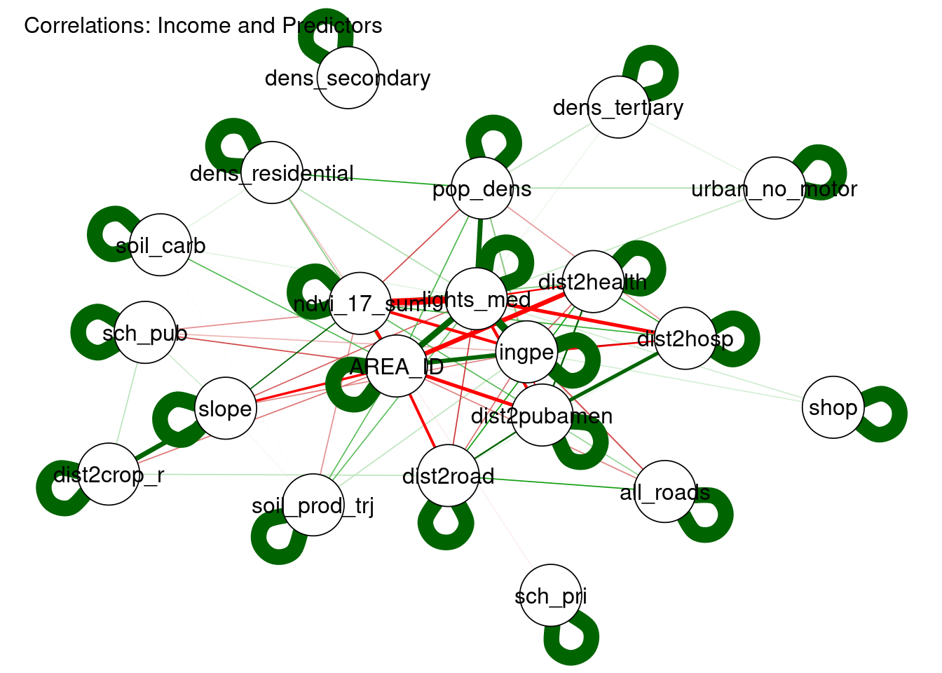
Figure 3.11: Correlogram of Income (ingpe) with Candidate Covariates
The plot in Fig.3.11 clearly shows that the top predictors are highly correlated.
3.3.2 Correlation with Literacy
The process described in the previous subsection is repeated for literacy.
Light at night is again the best predictor of literacy, by distance, the rural-urban segmento identifier, and normalized difference vegetation index (NDVI).
3.3.3 Correlation with Poverty
In examining this correlation, NDVI and distance to public amenities and hospitals, in particular, come first. We see that the level of correlation is lower than in the previous plot, suggesting that it might be harder to find good model fit for moderate poverty than for the other indicators.
Figure 3.12: Correlation of Candidate Covariates with Moderate Poverty
A Gaussian distribution is a normal distribution. We use the former terminology as it corresponds to the
INLAone↩︎