Section 6 Results summary
This section presents the results obtained with the models for the three development indicators: median income, literacy, and poverty rates. Goodness-of-fit statistics are presented both at the segmento level and at the municipio (municipal) level. In the latter case, the results are presented with models fitted on either the entire datasets or the 50 representative municipios only. Lastly, we present the map of predicted income, literacy, and poverty rates as well as the uncertainty maps.
6.1 Goodness of Fit at the Segmento Level
Various models were tested for the three development indicators. Spatial dependence was modeled either with a BYM 2 or an SPDE model. The backward selection process was adopted, starting from the same set of covariates. For the income model, we tested both Gaussian and gamma likelihood functions. Both literacy and poverty are ratio data, bounded between 0 percent and 100 percent, so we used a beta model. As beta distributions cannot include 0 and 1, we added and subtracted \(0.00001\) to observations with a 0 or 1, respectively. We also tested both models for the goodness of fit of a Gaussian model.
Additionally, we investigated the use of zero-inflated and zero-altered beta models for literacy and poverty. For poverty, we also tested two separate models for rural and urban segmentos, which did not yield any noticeable improvement in the model’s goodness of fit. We, therefore, do not present the codes and results for these more complex models.
The model summaries follow:
# Load the results ####
dir_result=paste0(root_dir,project_dir,"out/results/")
results_list=dir(dir_result)

for(i in 1:length(results_list)){
  load(paste0(dir_result,
              results_list[i]))
}

results_names=gsub(".RData","",results_list)
lines_r=list()
i=1
for(i in 1:length(results_names)){
  lines_r[[i]]=list(get(results_names[i])[[c("outcome")]],
                   get(results_names[i])[[c("spat_dep")]],
                   get(results_names[i])[[c("family")]],
                   get(results_names[i])[[c("cov_select")]],
                   get(results_names[i])[[c("r2_train")]],
                   get(results_names[i])[[c("r2_val")]],
                   get(results_names[i])[[c("r2_test")]],
                   get(results_names[i])[[c("RMSE_train")]],
                   get(results_names[i])[[c("RMSE_val")]],
                   get(results_names[i])[[c("RMSE_test")]])

  if(is.null(lines_r[[i]][[7]])){lines_r[[i]][[7]]=NA}
  if(is.null(lines_r[[i]][[10]])){lines_r[[i]][[10]]=NA}
  # print(length(lines_r[[i]]))
}
lines_df=do.call(rbind.data.frame, lines_r)
names(lines_df)=c("Outcome","spatial dependency model","likelihood","covariate selection method",
                  "r2 training set","r2 validation set","r2 test set",
                  "RMSE training set","RMSE validation set","RMSE test set")
Table 8.1 summarizes the RMSE and r-squared for the 10 models.
lines_df[,which(unlist(lapply(lines_df,is.numeric)))]=
  round(lines_df[,which(unlist(lapply(lines_df,is.numeric)))],digit=2)

caption_table='Summary of Goodness of Fit at the Segmento Level'
knitr::kable(
  lines_df,
  format="markdown",
  caption = caption_table,
  booktabs = TRUE,
row.names = FALSE)| Outcome | spatial dependency model | likelihood | covariate selection method | r2 training set | r2 validation set | r2 test set | RMSE training set | RMSE validation set | RMSE test set |
|---|---|---|---|---|---|---|---|---|---|
| illiteracy | bym2 | beta | naive | 0.65 | 0.43 | NA | 0.06 | 0.08 | NA |
| illiteracy_rate | spde | beta | naive | 0.53 | 0.42 | NA | 0.07 | 0.08 | NA |
| illiteracy_rate | spde | beta | stepwise | 0.55 | 0.46 | 0.43 | 0.07 | 0.07 | 0.08 |
| ingpe | bym2 | gamma | naive | 0.66 | 0.47 | NA | 42.25 | 63.76 | NA |
| ingpe | bym2 | gaussian | stepwise | 0.45 | 0.47 | 0.40 | 53.58 | 63.87 | 57.01 |
| ingpe | spde | gaussian | naive | 0.54 | 0.53 | NA | 0.32 | 0.33 | NA |
| ingpe | spde | gamma | naive | 0.48 | 0.48 | NA | 51.95 | 63.27 | NA |
| ingpe | spde | gamma | stepwise | 0.50 | 0.51 | 0.49 | 50.30 | 62.06 | 52.79 |
| pobreza_mod | bym2 | beta | naive | 0.62 | 0.25 | NA | 0.13 | 0.17 | NA |
| pobreza_mod | spde | beta | naive | 0.31 | 0.18 | NA | 0.17 | 0.18 | NA |
| pobreza_mod | spde | gaussian | stepwise | 0.31 | 0.30 | 0.24 | 0.17 | 0.18 | 0.19 |
| pobreza_mod | spde | beta | stepwise | 0.29 | 0.28 | 0.20 | 0.17 | 0.18 | 0.19 |
For income, the best model is the SPDE with a gamma likelihood function where stepwise covariate selection has been applied. The goodness of fit is relatively high (50 percent) and holds in the testing set.
For literacy, the three tested models yield results that are very close in terms of the goodness of fit. We select the SPDE with stepwise covariate selection, with a goodness of fit of 43 percent, as the final model.
However, the goodness of fit on the model on moderate poverty is only 23 percent. We select the Gaussian with SPDE and stepwise selection as the final model.
## OGR data source with driver: ESRI Shapefile
## Source: "/home/rstudio/data/spatial/shape/admin/STPLAN_Segmentos.shp", layer: "STPLAN_Segmentos"
## with 12435 features
## It has 17 fields
Figures 6.1, 6.2, and 6.3 show the predicted and observed values along with the \(R^{2}\) and the RMSE.
plotly::plot_ly(y=income_spde_stepwise$fit[income_spde_stepwise$index_train],
                x=ehpm17_predictors_nona$ingpe[income_spde_stepwise$index_train],
                type="scatter",
                mode="markers",
                name="training set",
                marker = list(color = 'black',
                              opacity = 0.3))%>%
  plotly::add_trace(y=income_spde_stepwise$fit[income_spde_stepwise$index_test],
                    x=ehpm17_predictors_nona$ingpe[income_spde_stepwise$index_test],
                    mode="markers",
                    name="test set",
                    marker = list(color = 'red',
                                  opacity = 0.3))%>%
  plotly::add_trace(y=c(0,880),
                    x=c(0,880),
                    type="scatter",
                    mode="lines",
                    name="1:1")%>%
  plotly::layout(yaxis=list(range=c(0,510),title="Predicted (USD)"),
                 xaxis=list(range=c(0,880),title="Observed (USD)"),
                 annotations=a,
                 title="Goodness of Fit: Income at the Segmento Level")
## A marker object has been specified, but markers is not in the mode
## Adding markers to the mode...Figure 6.1: Predicted versus Observed Income (USD), SPDE Model Stepwise Selection
Figure 6.2: Predicted versus Observed Median Income (USD), SPDE Model Stepwise Selection
Figure 6.3: Predicted versus Observed Moderate Poverty (%), SPDE Model Stepwise Selection
6.2 Segmento-Level Map
The detailed process to produce the maps is shown for income with the SPDE model. Codes are not shown for literacy and poverty. So far, predictions have been made on only the segmentos for which EHPM data are available, which is 1,664 segmentos. To complete the map, predictions have to be made on all of El Salvador’s 12,435 segmentos.
We prepare two data stacks: one covers the 1,664 EHPM segmentos and the other, the remaining 10,771 with no available EHPM data. For the latter segmentos, we do have the covariates data. The model will be trained on the EHPM segmentos, and out-of-sample prediction will be made on the non-EHPM segmentos.
load(paste0(dir_data,"workspace/income_spde_gamma.RData"))
data_model=segmento_sh_data_model@data

index_ehpm=which(is.na(data_model$ingpe)==F)
index_NON_ehpm=which(is.na(data_model$ingpe))

coords.ehpm=coordinates(segmento_sh_subset)
segmento_non_ehpm=subset(segmento_sh_data,
                         is.na(segmento_sh_data$ingpe))
coords.non.ehpm=coordinates(segmento_non_ehpm)


A.ehpm <- inla.spde.make.A(mesh=SV.mesh, loc=coords.ehpm)
A.non.ehpm <- inla.spde.make.A(mesh=SV.mesh, loc=coords.non.ehpm)


stack.ehpm= inla.stack(data = list(pred=data_model$ingpe[index_ehpm]),
                       A = list(A.ehpm, 1,1),
                       effects = list(s.index,
                                      Intercept=rep(1,length(index_ehpm)),
                                      data_model[index_ehpm,
                                                                   as.character(cov_candidates_selected_table$Candidates)]),
                       tag="ehpm")

stack.non.ehpm= inla.stack(data = list(pred=data_model$ingpe[index_NON_ehpm]),
                       A = list(A.non.ehpm, 1,1),
                       effects = list(s.index,
                                      Intercept=rep(1,length(index_NON_ehpm)),
                                      data_model[index_NON_ehpm,
                                                                   as.character(cov_candidates_selected_table$Candidates)]),
                       tag="non_ehpm")

join.stack <- inla.stack(stack.ehpm, stack.non.ehpm)
The model is now fitted with the usual inla command.
start_time=Sys.time()
M_map =inla(formula_selected,
            data=inla.stack.data(join.stack, spde=SV.spde),
            family="gamma",
            control.predictor=list(A=inla.stack.A(join.stack),
                                   link=1,compute=T),
            control.compute=list(cpo=F, dic=F))
end_time=Sys.time()
print(end_time-start_time)
## Time difference of 15.59154 secsThe fitted values are accessed using the inla.stack.index introduced in previous sections. We also extract the standard deviation of the prediction to map the uncertainty of the prediction. The latter is summarized by the coefficient of variation. For any given segmento \(s\), the coefficient of variation is given as
\[ \begin{aligned} coef var_{s}=\hat{\sigma_{s}}/\hat{\mu_{s}} \end{aligned} \] where \(\hat{\sigma_{s}}\) is the standard deviation of the prediction for segmento \(s\) and \(\hat{\mu_{s}}\) is the average predicted income for segmento \(s\). The coefficient of variation is the standard deviation of the prediction expressed as a percentage of the prediction.
index_inla_ehpm = inla.stack.index(join.stack,"ehpm")$data
index_inla_non_ehpm = inla.stack.index(join.stack,"non_ehpm")$data

M_map_fit=M_map$summary.fitted.values[,"mean"]

M_map_fit_ehpm=M_map$summary.fitted.values[index_inla_ehpm,"mean"]
M_map_fit_non_ehpm=M_map$summary.fitted.values[index_inla_non_ehpm,"mean"]
M_map_sd_ehpm=M_map$summary.fitted.values[index_inla_ehpm,"sd"]
M_map_sd_non_ehpm=M_map$summary.fitted.values[index_inla_non_ehpm,"sd"]
The fitted values, standard deviations, and coefficient of variations are now stored in the polygon data frame segmento_sh_data_model.
segmento_sh_data_model@data$fit_income=NA
segmento_sh_data_model@data$fit_income[index_ehpm]=M_map_fit_ehpm
segmento_sh_data_model@data$fit_income[index_NON_ehpm]=M_map_fit_non_ehpm

segmento_sh_data_model@data$sd_income=NA
segmento_sh_data_model@data$sd_income[index_ehpm]=M_map_sd_ehpm
segmento_sh_data_model@data$sd_income[index_NON_ehpm]=M_map_sd_non_ehpm

segmento_sh_data_model@data$coefvar_income=segmento_sh_data_model@data$sd_income/segmento_sh_data_model@data$fit_income
We can then save the spatial polygon data frame into a .geojson file for later inspection.
segmento_wgs_income=sp::spTransform(segmento_sh_data_model,
                            "+proj=longlat +datum=WGS84 +no_defs +ellps=WGS84 +towgs84=0,0,0")

segmento_wgs_income@data=segmento_wgs_income@data%>%
  select(SEG_ID,AREA_ID,fit_income,ingpe,sd_income,coefvar_income,lights_med,pop_dens,slope,n_obs)


rgdal::writeOGR(segmento_wgs_income_sp,
                paste0(dir_data,
                       "out/map/segmentos_spde_income2.geojson"),
                driver = "GeoJSON",
                layer = 1,
                overwrite_layer=T)
Figure 6.4 shows the map of the predicted income with a continuous color scale as well as the map of prediction uncertainty.4
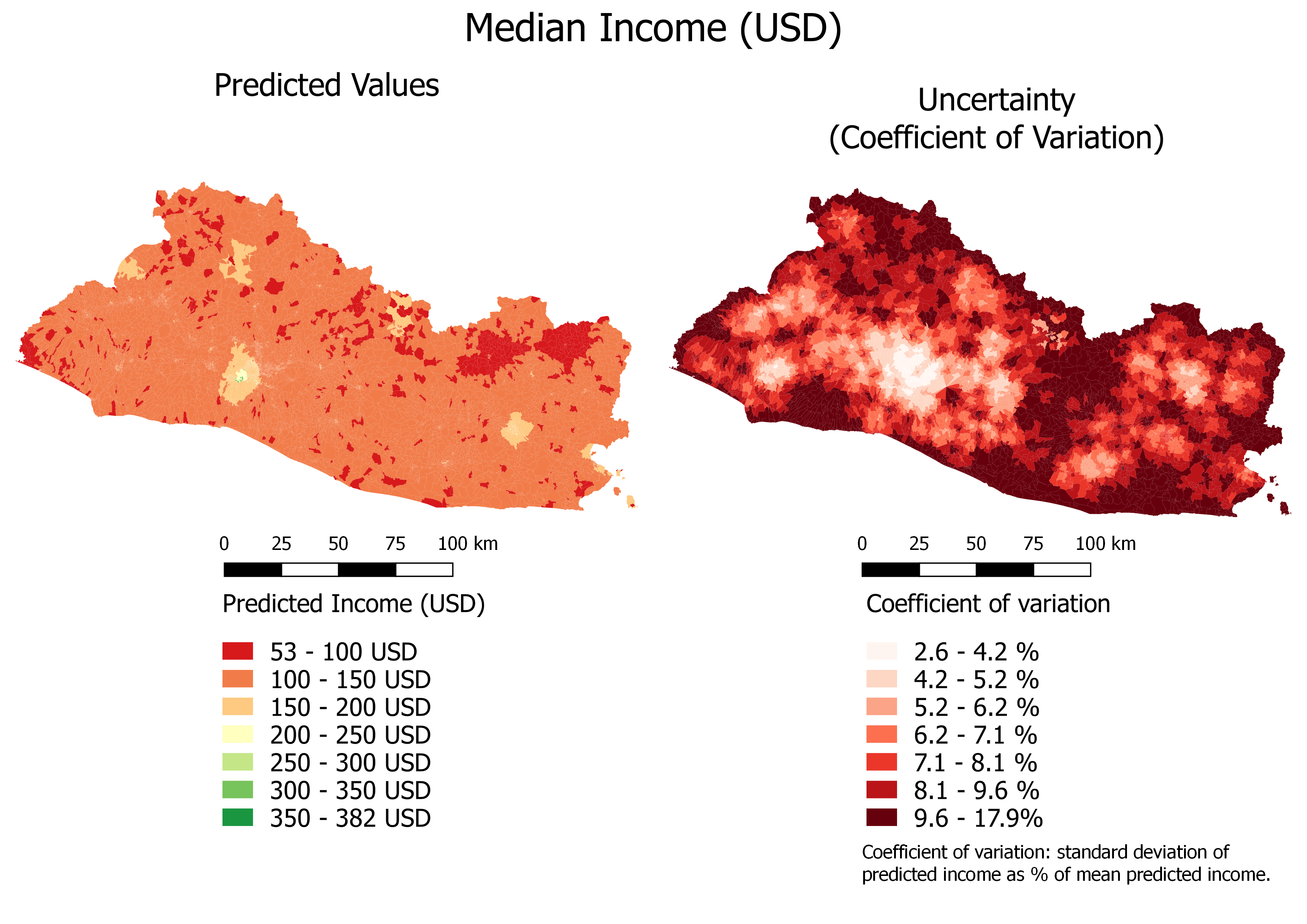
Figure 6.4: Median Income (USD): Continuous Color Scale
The prediction uncertainty is relatively low. In most cases, the coefficient of variation indicates that the standard deviation is smaller than 10 percent of the estimates.
Figure 6.5 shows the map of the predicted income with a quantile color scale, highlighting the rural-urban difference.
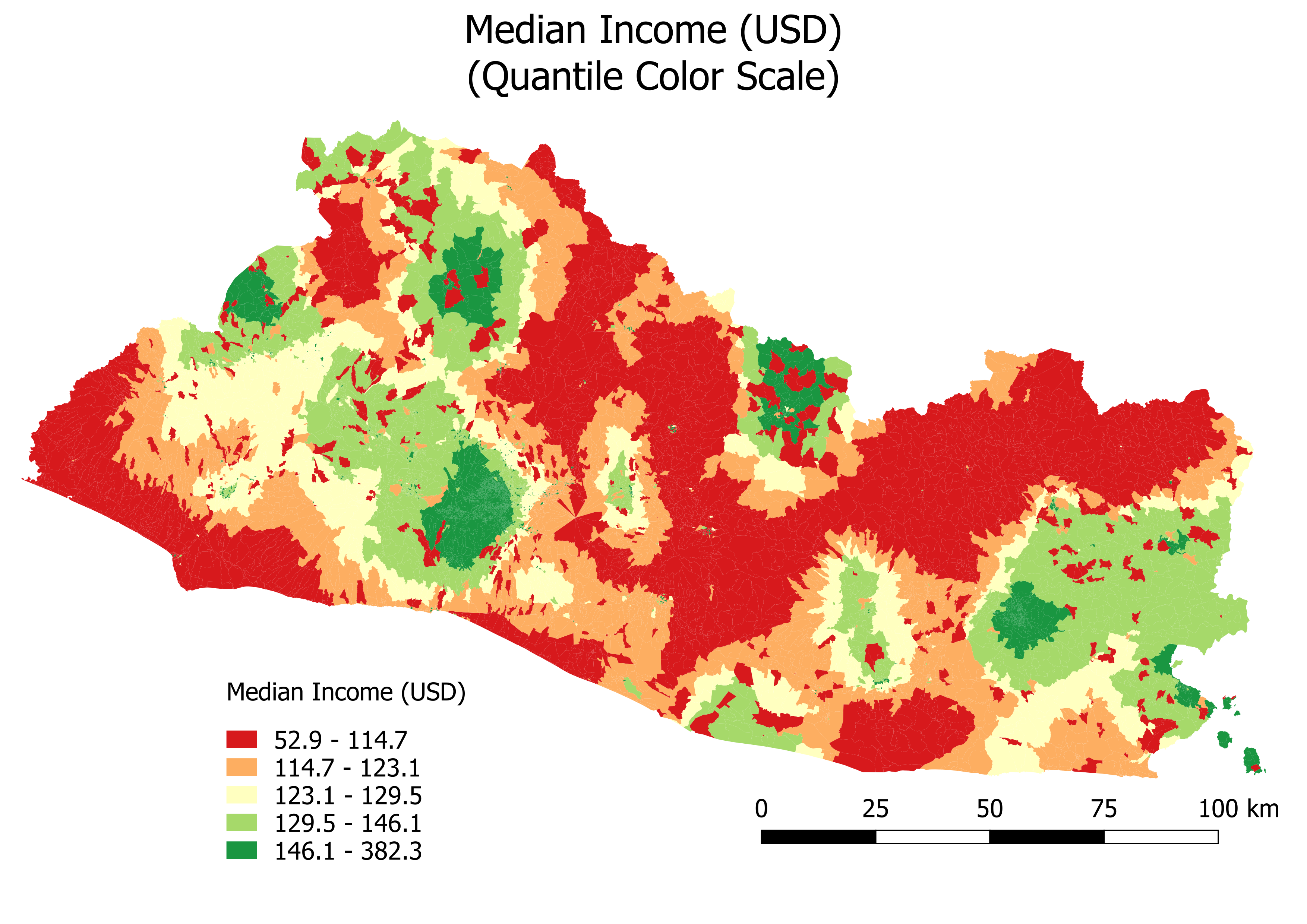
Figure 6.5: Median Income (USD): Quantile Color Scale
Figure 6.6 shows predicted illiteracy with a continuous color scale and uncertainty, while Figure 6.7 shows predicted illiteracy with a quantile color scale.
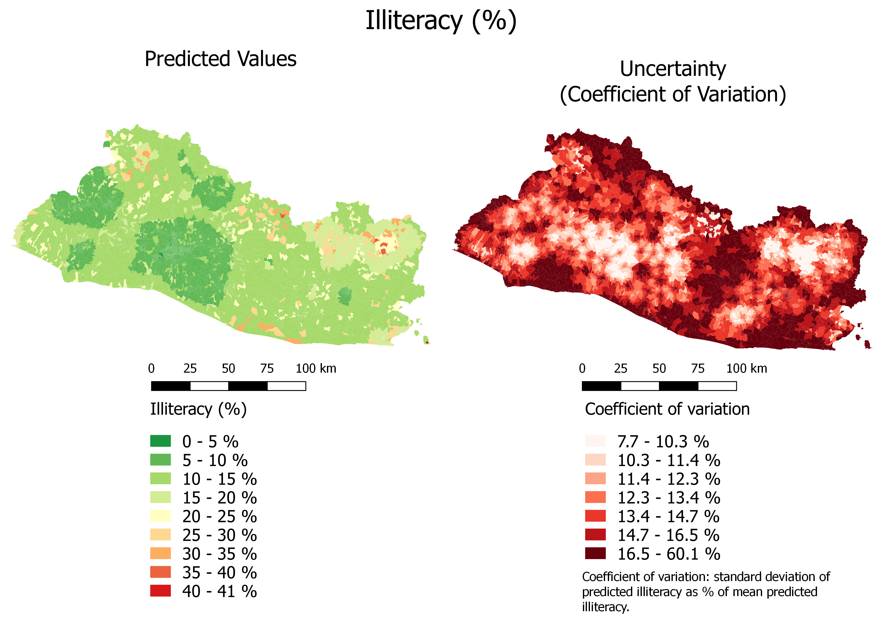
Figure 6.6: Illiteracy (%): Continuous Color Scale
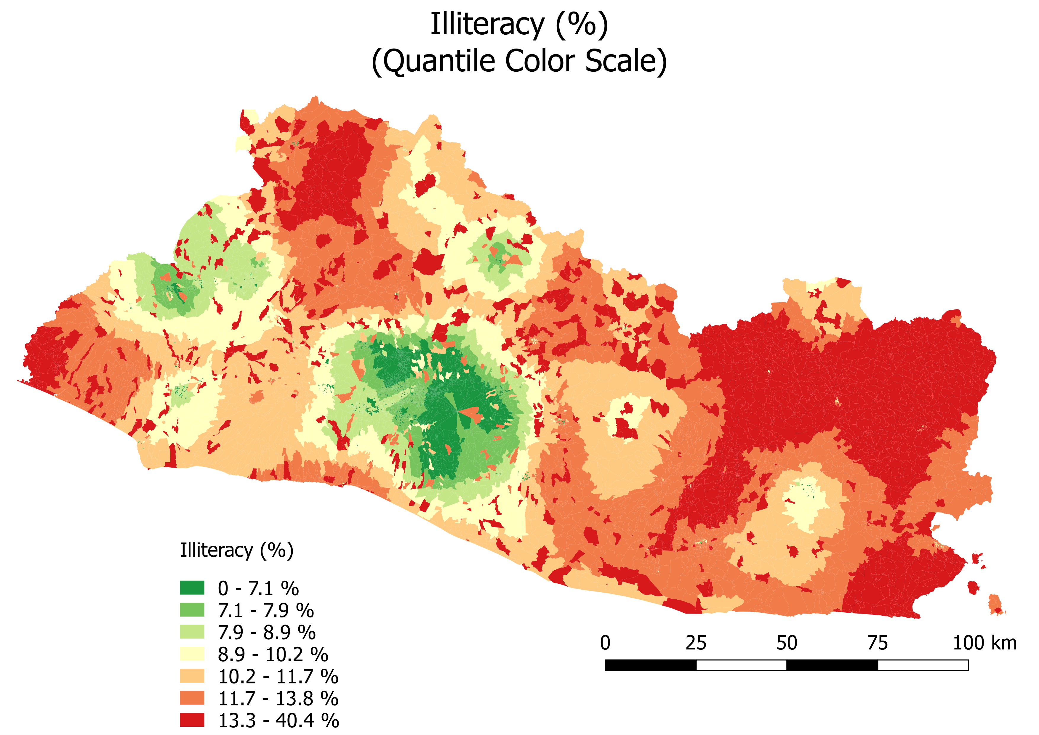
Figure 6.7: Illiteracy (%): Quantile Color Scale
Lastly, Figure 6.8 and Figure 6.9 show the results for moderate poverty.
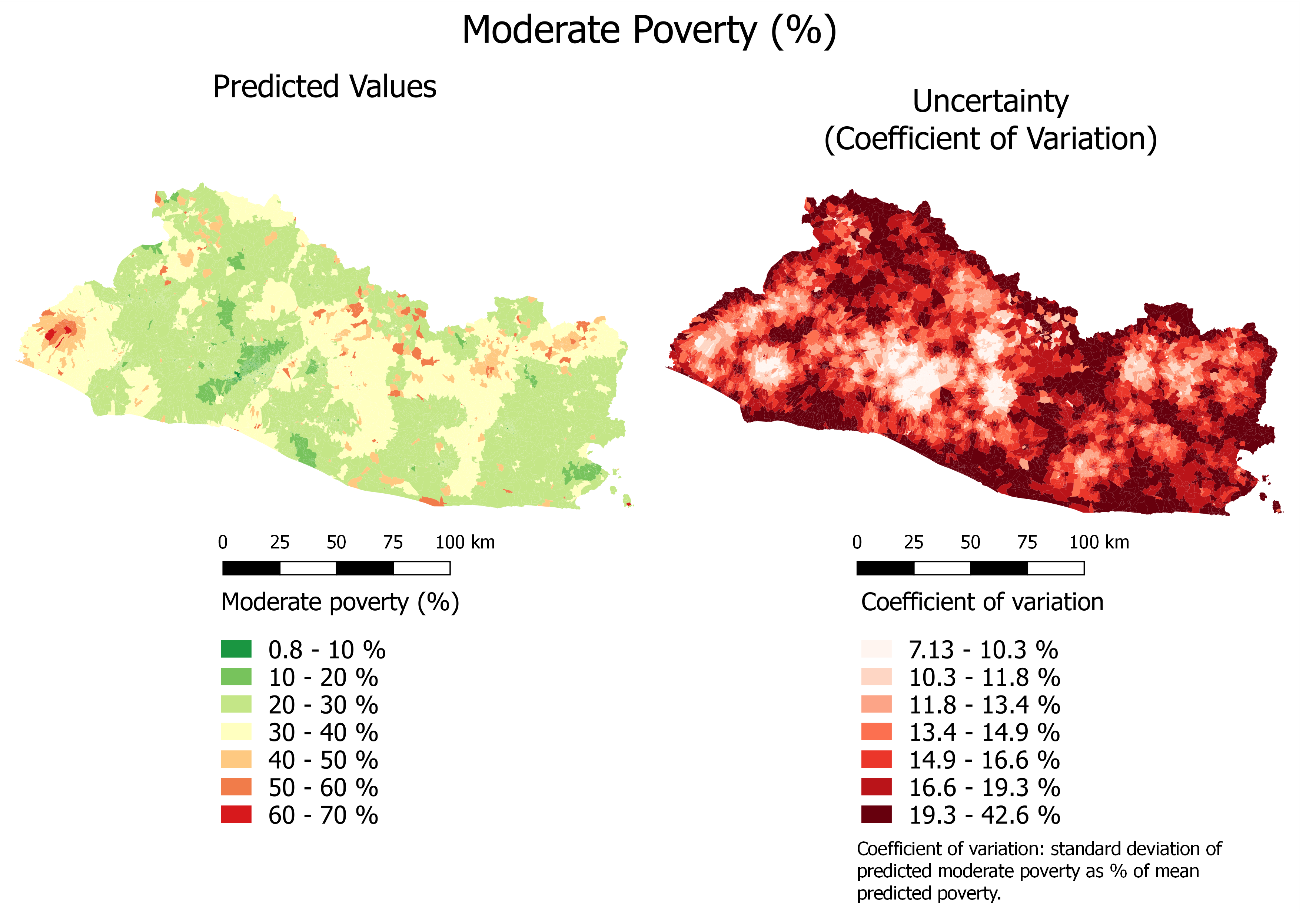
Figure 6.8: Moderate Poverty (%): Continuous Color Scale
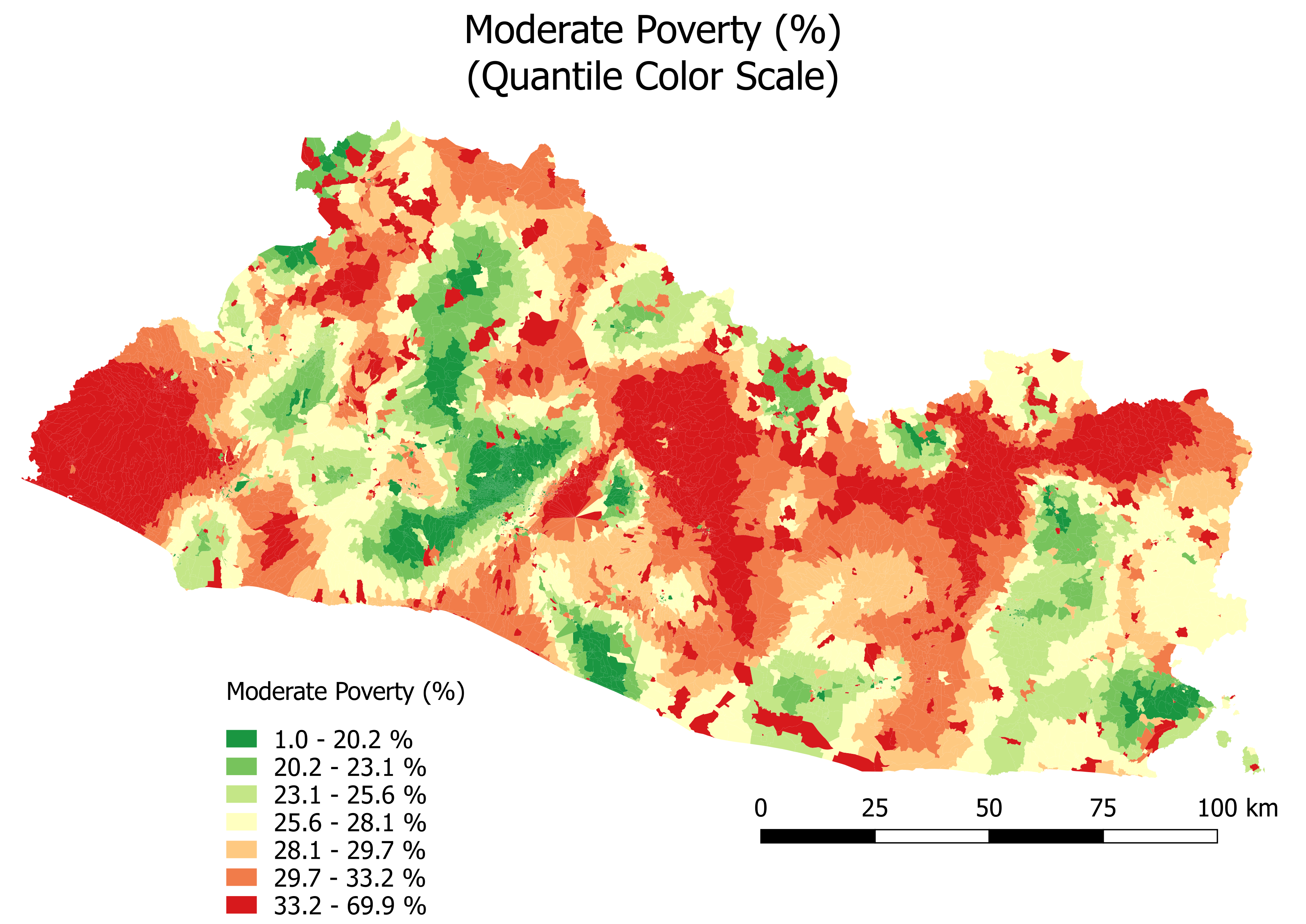
Figure 6.9: Moderate Poverty (%): Quantile Color Scale
6.3 Goodness of Fit at the Municipio Level
We now adopt two methods to investigate the goodness of fit at the municipio level.
First, we aggregate the results at the municipio level and compare them with municipio-level statistics. An issue with this approach is that in each municipio, some segmentos are used in the training and validation sets. Furthermore, EHPM data are representative at the municipio level only for a subset of municipios. Therefore, the difference between the fitted and observed values will be affected by both modeling and sampling errors, and it will be hard to gauge the external validity of the model because the training and validation sets are mixed.
To remedy this, we adopt a second approach. We select the segmentos from representative municipios only and split this remaining dataset into training and validation sets, making sure that all segmentos from any given municipio fall in either the training or the validation set. We can then obtain goodness-of-fit statistics at the municipio level for observations that have not been used to train the model.
6.3.1 Option 1: Aggregate the Results at the Municipio Level Using All Segmentos
First, we compute the average median income level per segmento on the entire sample at the municipio level. We then compute the average prediction of the test set at the municipio level. Finally, we compare the observed average income against the predicted average income at the municipio level, for both the representative and non-representative municipios.
# Reload the shape
source("../utils.R")
segmento_sh=rgdal::readOGR(paste0(dir_data,
                                  "spatial/shape/admin/STPLAN_Segmentos.shp"))
## OGR data source with driver: ESRI Shapefile
## Source: "/home/rstudio/data/spatial/shape/admin/STPLAN_Segmentos.shp", layer: "STPLAN_Segmentos"
## with 12435 features
## It has 17 fieldsehpm17_predictors=read.csv(paste0(dir_data,
"out/all_covariates_and_outcomes.csv"))
ehpm17_predictors=ehpm17_predictors%>%
mutate(SEG_ID=as.character(SEG_ID),
SEG_ID=ifelse(nchar(SEG_ID)==7,
paste0(0,SEG_ID),
SEG_ID))
# Extract the municipio identifier from the shapefile
segmento_sh_data=segmento_sh
segmento_sh_data@data=segmento_sh_data@data%>%
# dplyr::select(SEG_ID)%>%
mutate(SEG_ID=as.character(SEG_ID))%>%
left_join(ehpm17_predictors,
by="SEG_ID")
# Identify instances of EHPM data
segmento_sh_subset=subset(segmento_sh_data,
is.na(segmento_sh_data@data$ingpe)==F)
segmento_sh_subset$fit=NA
segmento_sh_subset$fit[income_spde_stepwise$index_train]=income_spde_stepwise$fit[income_spde_stepwise$index_train]
segmento_sh_subset$fit[income_spde_stepwise$index_val]=income_spde_stepwise$fit[income_spde_stepwise$index_val]
segmento_sh_subset$fit[income_spde_stepwise$index_test]=income_spde_stepwise$fit[income_spde_stepwise$index_test]
data_municipio=segmento_sh_subset@data%>%
select(SEG_ID,fit,ingpe)%>%
left_join(segmento_sh_data@data%>%
select(SEG_ID,DEPTO,MPIO)%>%
mutate(DEPTO_MPIO=paste0(DEPTO,MPIO))%>%
select(-c(DEPTO,MPIO)),
by="SEG_ID")
# Extract the representative information from the EHPM
ehpm=read.csv(paste0(dir_data,
"tables/ehpm-2017.csv"))
segID=readxl::read_xlsx(paste0(dir_data,
"tables/Identificador de segmento.xlsx"),
sheet="2017")
ehpm_municauto=ehpm%>%
select(r005,autorrepresentado,idboleta)%>%
left_join(segID,
by="idboleta")%>%
rename("SEG_ID"="seg_id")%>%
group_by(SEG_ID)%>%
summarise(autorrepresentado=mean(autorrepresentado))
# Add representativity indicator to results data frame
data_municipio_rep=data_municipio%>%
left_join(ehpm_municauto,
by="SEG_ID")
# Aggregate the results at the municipio level ####
# All
data_municipio_all=data_municipio_rep%>%
group_by(DEPTO_MPIO)%>%
summarise(obs=mean(ingpe,na.rm=T),
fit=mean(fit,na.rm=T))%>%
mutate(representative="all")
# Non-representative
data_municipio_NONREP=data_municipio_rep%>%
filter(autorrepresentado==0)%>%
group_by(DEPTO_MPIO)%>%
summarise(obs=mean(ingpe,na.rm=T),
fit=mean(fit,na.rm=T))%>%
mutate(representative="no")
# Representative
data_municipio_REP=data_municipio_rep%>%
filter(autorrepresentado==1)%>%
group_by(DEPTO_MPIO)%>%
summarise(obs=mean(ingpe,na.rm=T),
fit=mean(fit,na.rm=T))%>%
mutate(representative="yes")
# Bind the data frame
data_municipio=data_municipio_REP%>%
bind_rows(data_municipio_NONREP)%>%
bind_rows(data_municipio_all)
index_rep=which(data_municipio$representative=="yes")
index_non_rep=which(data_municipio$representative=="no")
index_all=which(data_municipio$representative=="all")
# Fit
RMSE=function(set,outcome,data,fit){
res = data[set,outcome]-fit[set]
RMSE_val <- sqrt(mean(res[,"obs"]^2,na.rm=T))
return(RMSE_val)
}
pseudo_r2=function(set,outcome,data,fit){
res = data[set,outcome]-fit[set]
RRes=sum((res)^2,na.rm = T)
RRtot=sum((data[set,outcome]-mean(fit[set],na.rm=T))^2,na.rm = T)
pseudo_r2_val=1-RRes/RRtot
return(pseudo_r2_val)
}
r2_all=pseudo_r2(index_all,"obs",data_municipio,data_municipio$fit)
r2_rep=pseudo_r2(index_rep,"obs",data_municipio,data_municipio$fit)
r2_non_rep=pseudo_r2(index_non_rep,"obs",data_municipio,data_municipio$fit)
RMSE_all=RMSE(index_all,"obs",data_municipio,data_municipio$fit)
RMSE_rep=RMSE(index_rep,"obs",data_municipio,data_municipio$fit)
RMSE_non_rep=RMSE(index_non_rep,"obs",data_municipio,data_municipio$fit)The results are plotted in Figure 6.10.
Figure 6.10: Predicted versus Observed Median Income: Municipio Level, Entire Sample
The results for literacy and poverty are shown in Figure 6.11 and Figure 6.12, respectively.
Figure 6.11: Predicted versus Observed Illiteracy Rate: Municipio Level, Entire Sample
Figure 6.12: Predicted versus Observed Moderate Poverty Rate: Municipio Level, Entire Sample
The goodness of fit is much better for the representative municipios (in green) than the non-representative ones (in red). In the latter ones, the goodness of fit is affected by both the model and sampling errors. Furthermore, it is hard to take the goodness-of-fit statistics for the representative segmentos at face value, as they are based on a mix of training and validation data. We accordingly rerun the model below with only the segmentos in representative municipios.
6.3.2 Option 2: Aggregate the Results at the Municipio Level Using Segmentos in Representative Municipios Only
We select only the segmentos in representative municipios and allocate the municipios to the training or validation set. This ensures that all segmentos from each municipio are in either the training or the validation set. There are 50 representative municipios in the EHPM totaling 1,114 segmentos.
The only change compared to the code shown in the earlier sections is the creation of the training and validation sets. The process is
- Allocate the representative municipios into training and validation sets.
- Select the data for the segmentos in the representative municipios.
- Add the municipio training and validation set indexes to the segment-level data frame.
# 1. Allocate the representative municipios into training and validation sets  ####
list_municipio=data_municipio_REP%>%
  distinct(DEPTO_MPIO)

set.seed(12345)
spec = c(train = .8, validate = .2)
g = sample(cut(
  seq(nrow(list_municipio)),
  nrow(list_municipio)*cumsum(c(0,spec)),
  labels = names(spec)
))

list_municipio$index=g

# 2. Select the data for the segmentos in the representative municipios ####
segmento_sh_data=segmento_sh

segmento_sh_data@data=segmento_sh_data@data%>%
  # dplyr::select(SEG_ID)%>%
  mutate(SEG_ID=as.character(SEG_ID))%>%
  left_join(ehpm17_predictors,
            by="SEG_ID")

segmento_sh_data@data=segmento_sh_data@data%>%
  mutate(DEPTO_MPIO=paste0(DEPTO,MPIO))
segmento_sh_subset_muni=subset(segmento_sh_data,
                               is.na(segmento_sh_data@data$ingpe)==F&
                                 segmento_sh_data@data$DEPTO_MPIO%in%list_municipio$DEPTO_MPIO) # identify where there is EHPM data and representative municipios

# 3. Add the municipio training and validation set indexes to the segment-level data frame
segmento_sh_subset_muni@data=segmento_sh_subset_muni@data%>%
  left_join(list_municipio,
            by="DEPTO_MPIO")

# Identify the indexes ####
index_train=which(segmento_sh_subset_muni$index=="train")
index_val=which(segmento_sh_subset_muni$index=="validate")
The rest of the process is the same: we create the mesh, the SPDE, the matrix of weights, the stack, the formula (we used the naive one), fit the model, and extract the fitted values (code not shown).
We then add the fitted values to the shapefile, aggregate the values at the municipio level, and compute separate goodness-of-fit statistics for the municipios in the training and validation sets.
# Add fitted values into the shapefile ####
segmento_sh_subset_muni@data$fit_income=NA
segmento_sh_subset_muni@data$fit_income[index_train]=results.train
segmento_sh_subset_muni@data$fit_income[index_val]=results.val

# Aggregate data at the municipio level ####
data_muni=segmento_sh_subset_muni@data%>%
  group_by(DEPTO_MPIO)%>%
  summarise(fit=mean(fit_income),
            obs=mean(ingpe),
            set=unique(index))
## `summarise()` ungrouping output (override with `.groups` argument)# Goodness of fit ####
RMSE=function(set,outcome,data,fit){
res = data[set,outcome]-fit[set]
RMSE_val <- sqrt(mean(res[,"obs"]^2,na.rm=T))
return(RMSE_val)
}
pseudo_r2=function(set,outcome,data,fit){
res = data[set,outcome]-fit[set]
RRes=sum((res)^2,na.rm = T)
RRtot=sum((data[set,outcome]-mean(fit[set],na.rm=T))^2,na.rm = T)
pseudo_r2_val=1-RRes/RRtot
return(pseudo_r2_val)
}
index_train_muni=which(data_muni$set=="train")
index_val_muni=which(data_muni$set=="validate")
r2_train_income=r2_train=pseudo_r2(index_train_muni,"obs",data_muni,data_muni$fit)
r2_val_income=r2_val=pseudo_r2(index_val_muni,"obs",data_muni,data_muni$fit)
RMSE_train_income=RMSE_train=RMSE(index_train_muni,"obs",data_muni,data_muni$fit)
RMSE_val_income=RMSE_val=RMSE(index_val_muni,"obs",data_muni,data_muni$fit)Figure 6.13: Predicted versus Observed Median Income: Municipio Level, Representative Municipios Only
The results for literacy and poverty are shown in Figure 6.14 and Figure @ref(fig: pobreza_mod-fit-municipio-2-chunk) respectively.
Figure 6.14: Predicted versus Observed Illiteracy: Municipio Level, Representative Municipios Only
(#fig:pobreza_mod-fit-municipio-2-chunk)Predicted versus Observed Moderate Poverty: Municipio Level, Representative Municipios Only
The three models’ goodness of fit at the municipio level is very high, as summarized in Table 8.2.
| Outcome | R-squared training (%) | R-squared validation (%) | RMSE training (USD) | RMSE validation (USD) |
|---|---|---|---|---|
| Median Income (USD) | 87.34 | 83.59 | 19.20 | 15.99 |
| Illiteracy (% of adults) | 72.90 | 77.60 | 0.03 | 0.03 |
| Moderate Poverty (% of adults) | 58.64 | 60.44 | 0.05 | 0.06 |
An option would have been to create an interactive map with the package
leaflet, but we chose to edit the map in QGIS and display it as an image to ease the rendering of the maps.↩︎