Section 4 Fitting a simple model
The goal of this section is to fit a simple model for income to introduce the modified Besag-York-Mollie model (BYM 2) and the stochastic partial differential equation (SPDE) model.
In both cases, the general process is the same:
- Define the spatial dependency.
- Split the model into training and validation sets.
- Specify the formula, expressing the outcome variables in terms of fixed and random spatial effects.
- Fit the model on the training set.
- Validate the model on the validation set.
The fixed effects are the covariates (e.g., population density or light at night). The spatial random effects are spatially correlated random effects used to model the spatial dependency.
Note that it is assumed here that the list of fixed effects is known. The next section presents a backward stepwise covariate selection process to select the list of covariates.
4.1 Loading the Data
We start by loading the covariates data and matching them with the segmento spatial polygon data frame.
rm(list=ls())
library(parallel)
library(INLA)
library(dplyr)
#INLA:::inla.dynload.workaround()

# Modify dir_data to where you stored the data
root_dir="~/"
project_dir="data/"

dir_data=paste0(root_dir,project_dir)

# Load the data ####
ehpm17_predictors=read.csv(paste0(dir_data,
                                  "out/all_covariates_and_outcomes.csv"))

# Correct for .xls misbehavior: The SEG_ID with a leading 0 were shortened (i.e. the leading 0 was eliminated)
ehpm17_predictors=ehpm17_predictors%>%
  mutate(SEG_ID=as.character(SEG_ID),
         SEG_ID=ifelse(nchar(SEG_ID)==7,
                       paste0(0,SEG_ID),
                       SEG_ID))

# Shape
segmento_sh=rgdal::readOGR(paste0(dir_data,
                                  "spatial/shape/admin/STPLAN_Segmentos.shp"))
## OGR data source with driver: ESRI Shapefile
## Source: "/home/rstudio/data/spatial/shape/admin/STPLAN_Segmentos.shp", layer: "STPLAN_Segmentos"
## with 12435 features
## It has 17 fields4.2 Area Data
4.2.1 Spatial Dependency with Area Data
To model the spatial dependency with data from the area data, we need to inform the model of neighboring segmentos.
The function spdep::poly2nb creates a neighbors list from the segmento polygon. The list is created in a spatial format suitable for INLA with the function spdep::nb2INLA. It is then read as a graph object for INLA consumption.
# Define neighboring structures ####
segmento_sh_data@data$ID=1:length(segmento_sh_data@data$n_obs)

segmento.nb=spdep::poly2nb(segmento_sh_data)
spdep::nb2INLA(paste0(dir_data,
                      "out/SEG.graph"),
               segmento.nb)
SEG.adj=paste0(paste0(dir_data,
                      "out/SEG.graph"),
               sep="")
Segmento.Inla.nb <- INLA::inla.read.graph(paste0(dir_data,
                                                 "out/SEG.graph"))
Figure 4.1 illustrates the results with data at the department level.
## OGR data source with driver: ESRI Shapefile
## Source: "/home/rstudio/data/spatial/shape/admin/STPLAN_Departamentos.shp", layer: "STPLAN_Departamentos"
## with 14 features
## It has 6 fields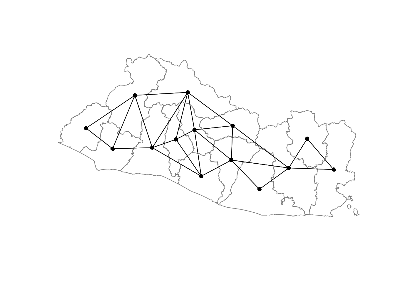
Figure 4.1: Neighboring Structures at the Departamento Level
4.2.2 Store the Data for Modeling
The data are stored in the data frame data_model.
# Identify EHPM 17 segmentos to fit the model ####
segmento_sh_data_model=segmento_sh_data

non_na_index=which(is.na(segmento_sh_data_model$n_obs)==F)

ehpm17_predictors_nona=segmento_sh_data_model@data[non_na_index,]


# Covariates #####
cov_candidates_selected_df=read.table(paste0(dir_data,
                                             "out/distance_corr_var/selected_all.txt"),
                                      header =T)
cov_candidates_selected_table=cov_candidates_selected_df
names(cov_candidates_selected_table)="Candidates"
# knitr::kable(
#   cov_candidates_selected_table,
#   caption = 'Candidate covariates for income',
#   booktabs = TRUE
# )
covariates=ehpm17_predictors_nona[,as.character(cov_candidates_selected_table$Candidates)]

# Store data for the model ####
data_model=data.frame(ingpe=ehpm17_predictors_nona$ingpe,
                      intercept=array(1,dim(covariates)[1]), # intercept for INLA
                      ID=ehpm17_predictors_nona$ID, # ID to link data to the neibhouring structure
                      covariates)
4.2.3 Split the Sample into 80-20 Training and Validation Sets
The observations in the dataset are split into 80-20 training and validation sets. The model will be fitted on the training set, and income will be predicted on the validation sets. The predicted values will be compared with the observed values of the validation set to assess the model’s goodness of fit.
# Take a sample of segmentos for training, validation, and test  ####
set.seed(1234)
spec = c(train = .8, validate = .2)
g = sample(cut(
  seq(nrow(data_model)),
  nrow(data_model)*cumsum(c(0,spec)),
  labels = names(spec)
))
index_val=which(g=="validate")
index_train=which(g=="train")

data_model$pred=data_model$ingpe
data_model$pred[c(index_val)] <- NA # Set the validation predictions NA: The values will be predicted by the model and compared with observed values
4.2.4 Formula Specifying the Relationship between the Outcome Variable and the Fixed and Spatial Random Effects
Next, we write a formula to predict income with a subset of the covariates and chose to use the following covariates:
- Binary indicator for rural and urban segmentos
- Median lights at night
- Population density
- Average slope in the segmentos
- Average precipitation
- Distance to public services
- Distance to businesses
- Distance to roads
# Write the test formula ####
formula_test =pred~
  AREA_ID+lights_med+pop_dens+slope+chirps_ev_2017+dist2pubamen+dist2road+
  f(ID,
    model = "bym2",
    graph = Segmento.Inla.nb,
    hyper=list(
      prec = list(prior = "pc.prec", param = c(0.1, 0.0001)),
      phi  = list(prior = "pc", param = c(0.5, 0.5))),
    scale.model = TRUE,
    constr = T,
    adjust.for.con.comp = T)
The variable pred is the output variable we aim to model (e.g., income).
The selected covariates are added linearly. Remember that they have been standardized in the previous section to avoid any issues linked to scale. These covariates are called fixed effects.
The most complex aspect of the formula is the spatial dependence structure specified in f().
The ID is the segmento identifiers linking the graph object Segmento.Inla.nb, where the neighboring structure is defined, with the data frame where the covariates and output data are stored. The model parameter is for the specification of the spatial correlation model that should be used. The bym2 is used because it is flexible and allows for a relatively intuitive specification of spatial random effects.
The flexibility comes from the fact that bym2 allows for the error term to be composed of two elements: (1) a pure random noise, and (2) a spatially correlated noise. The penalized complexity priors phi allows the importance of each effect to be influenced (if phi=0, then we have pure noise, if phi=1, we have only a spatially correlated random effect).
The prec parameter is the precision parameters, or how much the spatially correlated noise is allowed to vary spatially. If the value is high, then the spatially correlated noise is allowed to vary a lot across space and vice versa. By decreasing the penalized complexity priors on the precision parameter, we decrease the risk of overfitting: less of the spatial variation left unexplained by the covariates is attributed to the spatial random effects, and, as a result, the model is better able to generalize to areas where it was not trained.
Here, we have chosen to set the penalized complexity prior on precision as \(Pr(\sigma>1)=0.0001\) instead of the default \(Pr(\sigma>1)=0.01\). Indeed, we were facing overfitting issues with the default priors: the difference between the goodness of fit in the training and validation sets was very large (about 20 percent in the \(R^{2}\)).
4.2.5 Fit the Model on the Training Set
The model is fitted with the inla command. We have to specify the likelihood distribution of the response variable.
The family argument defines the type of likelihood function for the response variable. As the distribution of income is strictly positive and right skewed, a gamma distribution is a good option.
The data argument specifies the data on which the model is fitted, which in our case is the data_model data frame.
As we use a gamma likelihood function, the predicted values need to be back transformed to the original scale by using the exponential function. The control.predictor automatizes the process once the option list(link=1,compute=T) is specified.
We use a simple integration strategy to compute the posterior marginals of the model parameters by specifying control.inla =list(int.strategy = "eb"), where eb stands for “empirical Bayes.” In the empirical Bayes approach, we use only one “integration point equal to the posterior mode of the hyperparameters” (Moraga 2019). This speeds up the estimation of the model.
# Fit the model on the training set ####
start_time=Sys.time() # Time the start of the estimation
bym.res=inla(formula=formula_test,
             family = "gamma",
             data = data_model,
             control.predictor=list(link=1,compute=T),
             control.inla =list(int.strategy = "eb"))
end_time=Sys.time() # Time at the end of the estimation
duration=end_time-start_time
print(duration)
## Time difference of 54.15509 secsIt took 3.7 minutes to estimate the model. With the default integration strategy, the model takes 13.5 minutes to be estimated. No significant difference was found between the integration strategies.
4.2.6 Validate the Model on the Validation Set
The model’s goodness of fit can now be investigated on the validation set. We start by extracting the fitted values, which are stored in the bym.res object under summary.fitted.values. The inla model yields a distribution of predicted income for each segmento. Various statistics summarizing this prediction are also available for each segmento:
- The mean fitted value
- The median fitted value
- The 2.5 and 97.5 percentiles of the fitted values
- The standard deviation of the fitted value distribution
Below, we select the mean fitted value, that is, the mean prediction value for each segmento.
We can now compute the root mean square error (RMSE) and the pseudo \(R^{2}\) as shown below.2
RMSE=function(set,outcome,data,fit){
  res = data[set,outcome]-fit[set]
  RMSE_val <- sqrt(mean(res^2,na.rm=T))
  return(RMSE_val)
}

pseudo_r2=function(set,outcome,data,fit){
  res =  data[set,outcome]-fit[set]
  RRes=sum((res)^2,na.rm = T)
  RRtot=sum((data[set,outcome]-mean(fit[set],na.rm=T))^2,na.rm = T)
  pseudo_r2_val=1-RRes/RRtot
  return(pseudo_r2_val)
}

RMSE_val=RMSE(index_val,"ingpe",data_model,M_fit)
RMSE_train=RMSE(index_train,"ingpe",data_model,M_fit)

r2_val=pseudo_r2(index_val,"ingpe",data_model,M_fit)
r2_train=pseudo_r2(index_train,"ingpe",data_model,M_fit)
a <- list(
x = 600,
y = 100,
text = paste("R2 training set:",round(r2_train*100),"%",
"\nR2 validation set:",round(r2_val*100),"%",
"\n",
"\nRMSE training set:",round(RMSE_train),"USD",
"\nRMSE validation set:",round(RMSE_val),"USD"),
xref = "x",
yref = "y",
showarrow = F)Figure 4.2: Observed versus Predicted Income Values, BYM 2 Model
Figure 4.2 shows the predicted and observed income values for the training and validation sets. The model appears to do a relatively good job, although it has difficulty capturing the segmentos with an income above 400.
An \(R^{2}\) of 44 percent is relatively satisfactory. It means that 44 percent of the income variation in the validation set is explained by the model fitted on the training set. However, the fact that the \(R^{2}\) is at 69 percent, close to twice as large as the \(R^{2}\) in the validation set, indicates overfitting.
The RMSE is USD 66 in the validation set and USD 40 in the training set. The RMSE is the standard deviation of the residuals, the difference between the fitted and observed values.
The results are stored in a list and saved in a .RData file for later consumption.
income_bym2_naive=list("outcome"="ingpe",
                       "spat_dep"="bym2",
                       "cov_select"="naive",
                       "formula"=formula_test,
                       "family"="gamma",
                       "data"=data_model,
                       "fit"=M_fit,
                       "index_val"=index_val,
                       "index_train"=index_train,
                       "r2_val"=r2_val,
                       "r2_train"=r2_train,
                       "RMSE_val"=RMSE_val,
                       "RMSE_train"=RMSE_train)
save(income_bym2_naive,
     file=paste0(dir_data,
            "out/results/income_bym2_naive.RData"))
4.3 Point-Referenced Data
4.3.1 Spatial Dependency with Point-Referenced Data
The spatial dependence is modeled here with an SPDE approach. The following steps are required:
1 Create the mesh. 2 Create the SPDE. *3 Create the matrix of weights.
4.3.1.1 Create the Mesh
To create the mesh, we start by identifying the segmentos for which there are EHPM data. Second, we create a spatial polygon of the country’s boundaries by dissolving the shapefile of the departamentos with the function unionSpatialPolygons. Third, we transform this spatial polygon into a list that the INLA library can process with the function inla.sp2segment. Lastly, we use the helper function inla.mesh.create.helper to create the mesh, using the boundary and coordinates of the segmentos’ centroids (i.e., middle points) as inputs.
# Create the mesh ####
segmento_sh_subset=subset(segmento_sh_data_model,
                          is.na(segmento_sh_data_model@data$ingpe)==F) # Identify where there is EHPM data

coords=coordinates(segmento_sh_subset) # Collect the coordinates of the segmentos with EHPM data
SVborder <- maptools::unionSpatialPolygons(departamentos_sh,
                                           rep(1, nrow(departamentos_sh))) # Create one polygon using the boundaries of the countries
SV.bdry <- inla.sp2segment(SVborder) # Create an inla boundary object

SV.mesh <- inla.mesh.create.helper(
  boundary=SV.bdry,
  points=coords,
  offset=c(2500, 25000),
  max.edge=c(20000, 50000),
  min.angle=c(25, 25),
  cutoff=8000,
  plot.delay=NULL)
plot(SV.mesh,main="",asp=1)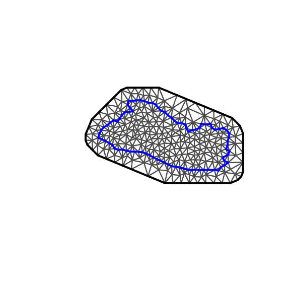
Figure 4.3: Mesh
The offset parameters of inla.mesh.create.helper define the inner and outer distances. For instance, if we change the outer offset parameter to 250 kilometers instead of the original 25 kilometers, the result is plotted in Figure 4.4.
SV.meshL <- inla.mesh.create.helper(
  boundary=SV.bdry,
  points=coords,
  offset=c(2500, 250000), # we increased from 25000 to 250000
  max.edge=c(20000, 50000),
  min.angle=c(25, 25),
  cutoff=8000,
  plot.delay=NULL)
plot(SV.meshL,main="",asp=1)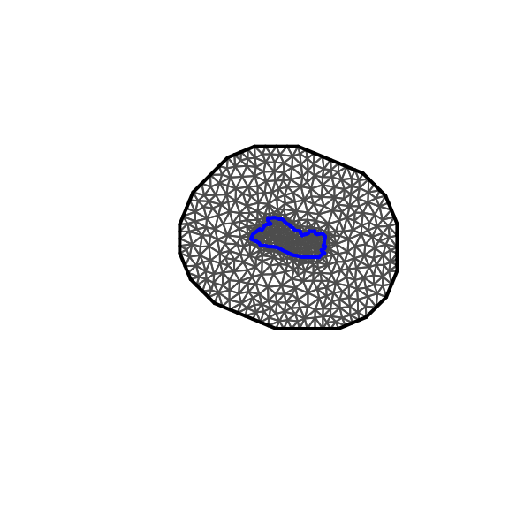
Figure 4.4: Mesh
When choosing the outer offset parameter, the aim is to avoid the presence of boundary effects in the subsequent estimation of the SPDE, so it is best to allow for a sufficient distance as shown in Figure 4.3. However, Figure 4.4 is clearly too large and would slow the estimation process.
The inner offset parameter has no effect here, as it is superseded by the max.edge, min.angle, and cutoff parameters. The max.edge parameter defines the largest-allowed triangle-edge length. The min.angle parameter defines the smallest-allowed triangle angle, and the parameter cutoff defines the minimum-allowed distance between points.
Next, we illustrate the impact of modifying the max.edge from 20 kilometers to 5 kilometers.
SV.meshL <- inla.mesh.create.helper(
  boundary=SV.bdry,
  points=coords,
  offset=c(2500, 25000),
  max.edge=c(20000, 5000), # Decrease from 50,000 to 5,000
  min.angle=c(25, 25),
  cutoff=8000,
  plot.delay=NULL)
plot(SV.meshL,main="",asp=1)
Figure 4.5: Mesh
Figure 4.5 shows the results. The risk of such a tight mesh is that it could lead to overfitting. Furthermore, it is computationally more expensive.
4.3.1.2 Derive the SPDE
Next, the SPDE is derived from the mesh using the inla.spde2.matern function, and the spatial index is derived with the function inla.spde.make.index.
# Create the SPDE ####
SV.spde <- inla.spde2.matern(mesh=SV.mesh,alpha=2)

s.index <- inla.spde.make.index(name="spatial.field", n.spde=SV.spde$n.spde)
The s.index allows the mesh to link to the matrix of spatial weights that will be defined below.
#### Create the matrix of weights
The matrix of weights is created with the INLA function inla.spde.make.A.
4.3.2 Store the Data for Modeling in a Stack
We use the inla.stack function to conveniently store the data in one object.
# Stack ####
covariates_list=c("AREA_ID","lights_med","pop_dens","slope","chirps_ev_2017","dist2pubamen","dist2road")
stack.train <- inla.stack(data = list(pred=segmento_sh_subset@data$ingpe[index_train]), # This output variable (income)
A = list(A.train, 1,1),
effects = list(s.index,
Intercept=1:length(index_train),
segmento_sh_subset@data[index_train,c(covariates_list)]),
tag="train") # The tag allows selected statistics for the desired sample to be extracted later
stack.val <- inla.stack(data = list(pred=NA), # Set it to NA
A = list(A.val, 1,1),
effects = list(s.index,
Intercept=1:length(index_val),
segmento_sh_subset@data[index_val,c(covariates_list)]),
tag="val")
# Combine both stacks
join.stack <- inla.stack(stack.train, stack.val)4.3.3 Specifying the Relationship between the Outcome Variable and the Fixed and Spatial Random Effects
We use the same set of fixed effects.
# Write the test formula ####
formula_test =pred~ -1+Intercept+
AREA_ID+lights_med+pop_dens+slope+chirps_ev_2017+dist2pubamen+dist2road+
f(spatial.field, model=SV.spde)The main difference from the BYM 2 specification is that the spatial random effects are specified by the f() function, which takes two arguments: spatial.field is the name of the spatial index s.index, and the model is the SPDE defined in SV.spde.
4.3.4 Fit the Model on the Training Set
The same inla command used to fit the areal model is used to fit the SPDE model. The only difference is that the data argument takes the stack data defined above as an input.
# Fit the model####
start_time=Sys.time()
spde_res=inla(formula_test, # Formula
data=inla.stack.data(join.stack),
family="gamma", # Likelihood of the data
control.predictor=list(A=inla.stack.A(join.stack),
link=1,compute=T))
end_time=Sys.time()
print(end_time-start_time) ## Time difference of 10.57809 secsThe model is much faster to fit: it took only 19 seconds (against 3.5 minutes for the BYM 2 model).
4.3.5 Validate the Model on the Validation Set
We can now investigate the model’s goodness of fit. To extract the fitted values for the training and validation sets from the income_spde_test object, we use the inla.stack.index function. Again, we extract only the mean predicted value for each segmento.
# Extract the fitted values
index_inla_train = inla.stack.index(join.stack,"train")$data
index_inla_val = inla.stack.index(join.stack,"val")$data
results.train=spde_res$summary.fitted$mean[index_inla_train]
results.val=spde_res$summary.fitted$mean[index_inla_val]
M_fit_spde=array(NA,length(M_fit))
M_fit_spde[index_train]=results.train
M_fit_spde[index_val]=results.val
r2_train_spde=pseudo_r2(index_train,"ingpe",segmento_sh_subset@data,M_fit_spde)
r2_val_spde=pseudo_r2(index_val,"ingpe",segmento_sh_subset@data,M_fit_spde)
rmse_train_spde=RMSE(index_train,"ingpe",segmento_sh_subset@data,M_fit_spde)
rmse_val_spde=RMSE(index_val,"ingpe",segmento_sh_subset@data,M_fit_spde)a <- list(
x = 600,
y = 100,
text = paste("R2 training set:",round(r2_train_spde*100),"%",
"\nR2 validation set:",round(r2_val_spde*100),"%",
"\n",
"\nRMSE training set:",round(rmse_train_spde),"USD",
"\nRMSE validation set:",round(rmse_val_spde),"USD"),
xref = "x",
yref = "y",
showarrow = F)Figure 4.6: Observed versus Predicted Income Values, SPDE Model
Figure 4.6 shows the observed values against the predicted values for the training and validation sets. There are no major differences in the results obtained with the modified BYM model shown in Figure 4.2 except that there does not appear to be overfitting here, as the \(R^{2}\) are similar in the training and validation sets.
Next, we save the results for later use.
income_spde_naive=list("outcome"="ingpe",
"spat_dep"="spde",
"cov_select"="naive",
"formula"=formula_test,
"family"="gamma",
"data"=join.stack,
"fit"=M_fit_spde,
"index_val"=index_val,
"index_train"=index_train,
"r2_val"=r2_val_spde,
"r2_train"=r2_train_spde,
"RMSE_val"=rmse_val_spde,
"RMSE_train"=rmse_train_spde)
save(income_spde_naive,
file=paste0(dir_data,
"out/results/income_spde_naive.RData"))Lastly, Figure 4.7 shows the results when using a Gaussian likelihood and log transforming the income data. There is a minor improvement to the goodness of fit compared to the gamma model.
# Write the test formula ####
formula_test =log(pred)~ -1+Intercept+
AREA_ID+lights_med+pop_dens+slope+chirps_ev_2017+dist2pubamen+dist2road+
f(spatial.field, model=SV.spde)
# Fit the model####
spde_res=inla(formula_test, # Formula
data=inla.stack.data(join.stack),
family="gaussian", # Likelihood of the data
control.predictor=list(A=inla.stack.A(join.stack),
link=1,compute=T))
# Extract the fitted values
index_inla_train = inla.stack.index(join.stack,"train")$data
index_inla_val = inla.stack.index(join.stack,"val")$data
results.train=spde_res$summary.fitted$mean[index_inla_train]
results.val=spde_res$summary.fitted$mean[index_inla_val]
M_fit_spde=array(NA,length(M_fit))
M_fit_spde[index_train]=results.train
M_fit_spde[index_val]=results.val
# Compute the goodness-of-fit statistics
segmento_sh_subset@data$ln_ingpe=log(segmento_sh_subset@data$ingpe)
r2_train_spde=pseudo_r2(index_train,"ln_ingpe",segmento_sh_subset@data,M_fit_spde)
r2_val_spde=pseudo_r2(index_val,"ln_ingpe",segmento_sh_subset@data,M_fit_spde)
rmse_train_spde=RMSE(index_train,"ln_ingpe",segmento_sh_subset@data,M_fit_spde)
rmse_val_spde=RMSE(index_val,"ln_ingpe",segmento_sh_subset@data,M_fit_spde)
a <- list(
x = 4,
y = 6,
text = paste("R2 training set:",round(r2_train_spde*100),"%",
"\nR2 validation set:",round(r2_val_spde*100),"%",
"\n",
"\nRMSE training set:",round(rmse_train_spde,1),"log USD",
"\nRMSE validation set:",round(rmse_val_spde,1),"log USD"),
xref = "x",
yref = "y",
showarrow = F)Figure 4.7: Observed versus predicted income values, SPDE model with Gaussian likelihood and Log-transformed income values
# Save the results
income_spde_naive_gaussian=list("outcome"="ingpe",
"spat_dep"="spde",
"cov_select"="naive",
"formula"=formula_test,
"family"="gaussian",
"data"=join.stack,
"fit"=M_fit_spde,
"index_val"=index_val,
"index_train"=index_train,
"r2_val"=r2_val_spde,
"r2_train"=r2_train_spde,
"RMSE_val"=rmse_val_spde,
"RMSE_train"=rmse_train_spde)
save(income_spde_naive_gaussian,
file=paste0(dir_data,
"out/results/income_spde_naive_gaussian.RData"))4.4 K-fold Cross-Validation
The split of the observations between the training and validation sets has an important impact on the model’s goodness of fit. Indeed, the model could fit the training set observations very well but the validations set observations so poorly as to fit them purely by chance.
K-fold cross-validation is a way to assess the results’ robustness to various splits of the data. In K-fold cross-validation, the data a split in K folds, and each fold is used only once for validation purposes and \(K-1\) times for training purposes. At the end of the validation process, one can assess how the goodness-of-fit statistics vary and the stastistics’ average value. A typical value for K is 10.
The 10 folds are created as follows:
set.seed(1)
spec = c(val1 = .1, val2 = .1, val3 = .1,
val4 = .1, val5 = .1, val6 = .1,
val7 = .1, val8 = .1, val9 = .1,
val10 = .1)
g = sample(cut(
seq(nrow(data_model)),
nrow(data_model)*cumsum(c(0,spec)),
labels = names(spec)
))We then fit the model 10 times, using each fold as a validation set once.
r2_train_spde_a=r2_val_spde_a=rmse_train_spde_a=rmse_val_spde_a=c() # Prepare empty array to store goodness-of-fit statistics
for(k in 1:10){
# Define the index
index_val=which(g==paste0("val",k))
index_train=which(g!=paste0("val",k))
# Define the weights
A.train <- inla.spde.make.A(mesh=SV.mesh, loc=coords[index_train,])
A.val <- inla.spde.make.A(mesh=SV.mesh, loc=coords[index_val,])
# Build the stack
covariates_list=c("AREA_ID","lights_med","pop_dens","slope","chirps_ev_2017","dist2pubamen","dist2road")
stack.train <- inla.stack(data = list(pred=segmento_sh_subset@data$ingpe[index_train]), # This output variable (income)
A = list(A.train, 1,1),
effects = list(s.index,
Intercept=1:length(index_train),
segmento_sh_subset@data[index_train,c(covariates_list)]),
tag="train") # The tag allows selected statistics for the desired sample to be extracted later
stack.val <- inla.stack(data = list(pred=NA), # Set it to NA
A = list(A.val, 1,1),
effects = list(s.index,
Intercept=1:length(index_val),
segmento_sh_subset@data[index_val,c(covariates_list)]),
tag="val")
join.stack <- inla.stack(stack.train, stack.val)
# Write the test formula ####
formula_test =pred~ -1+Intercept+
  AREA_ID+lights_med+pop_dens+slope+chirps_ev_2017+dist2pubamen+dist2road+
  f(spatial.field, model=SV.spde)
# Fit the model
spde_res=inla(formula_test, # formula
data=inla.stack.data(join.stack),
family="gamma", # likelihood of the data
control.predictor=list(A=inla.stack.A(join.stack),
link=1,compute=T))
end_time=Sys.time()
# Extract the fitted values
index_inla_train = inla.stack.index(join.stack,"train")$data
index_inla_val = inla.stack.index(join.stack,"val")$data
results.train=spde_res$summary.fitted$mean[index_inla_train]
results.val=spde_res$summary.fitted$mean[index_inla_val]
M_fit_spde=array(NA,length(M_fit))
M_fit_spde[index_train]=results.train
M_fit_spde[index_val]=results.val
# Compute goodness-of-fit statistics
r2_train_spde=pseudo_r2(index_train,"ingpe",segmento_sh_subset@data,M_fit_spde)
r2_val_spde=pseudo_r2(index_val,"ingpe",segmento_sh_subset@data,M_fit_spde)
rmse_train_spde=RMSE(index_train,"ingpe",segmento_sh_subset@data,M_fit_spde)
rmse_val_spde=RMSE(index_val,"ingpe",segmento_sh_subset@data,M_fit_spde)
# Store goodness-of-fit statistics in an array
r2_train_spde_a=c(r2_train_spde_a,r2_train_spde)
r2_val_spde_a=c(r2_val_spde_a,r2_val_spde)
rmse_train_spde_a=c(rmse_train_spde_a,rmse_train_spde)
rmse_val_spde_a=c(rmse_val_spde_a,rmse_val_spde)
# Print status
# Print(paste(k, "folds done"))
}
print(paste("Average R2 in the validation set:", round(mean(r2_val_spde_a)*100),"%",
"\nAverage R2 in the training set:", round(mean(r2_train_spde_a)*100),"%"))## [1] "Average R2 in the validation set: 44 % \nAverage R2 in the training set: 48 %"The average \(R^{2}\) of the validation and training sets (respectively 41 percent and 47 percent) are in line with the results obtained with the original split.
References
Moraga, P. 2019. Geospatial Health Data: Modeling and Visualization with R-Inla and Shiny. Chapman & Hall/CRC Biostatistics Series.
We refer to the pseudo \(R^{2}\) as the \(R^{2}\) in the report. The pseudo \(R^{2}\) is preferred to the normal \(R^{2}\) (squared correlation between the fitted and observed values), as it allows for better comparison with nonlinear models.↩︎